How to Use Currency Formatting in Google Sheets (and Remove the Dollar Sign)

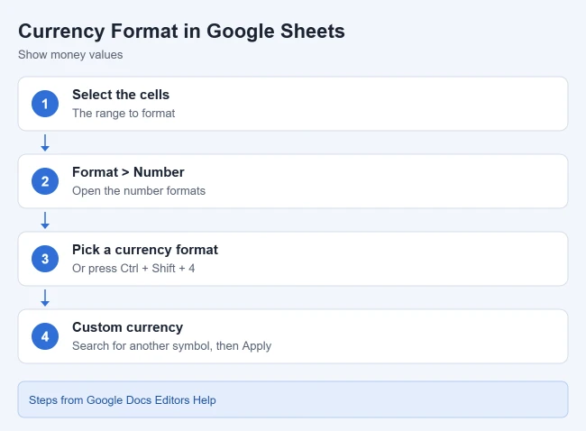
To use currency formatting in Google Sheets, select the cells, click Format > Number, and choose a currency format. The keyboard shortcut is Ctrl + Shift + 4. To remove the dollar sign, select the same cells and click Format > Number > Number. The amounts stay the same; only the symbol goes away.

These steps follow Google’s current help pages for Google Sheets in a desktop web browser, with separate steps for the Android and iPhone or iPad apps. You need edit access to the spreadsheet. If you can only view or comment, the formatting options are not available to you.

What Currency Formatting Does

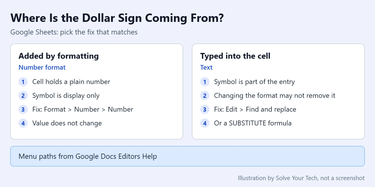
A number format changes how a value is displayed, not the value itself. When a cell that holds 1250.5 is formatted as currency, Sheets shows something like $1,250.50, but formulas still work with the plain number underneath. That is why you can add and remove the dollar sign as often as you like without changing your totals.

The symbol Sheets uses by default comes from the spreadsheet’s locale, which is the country or region setting for the file. A spreadsheet set to the United States uses the dollar sign.

How to Apply Currency Formatting on a Computer

1. Open your spreadsheet in Google Sheets.
2. Select the cells you want to format. Click one cell, drag across a range, or click a column letter to select the whole column.
3. Click Format in the menu bar at the top of the window.
4. Click Number. A list of number formats opens.
5. Click a currency format in the list.

The selected cells now show a currency symbol in front of each number. Numbers you type into those cells later pick up the same format.

For a faster route, select the cells and press Ctrl + Shift + 4, which Google lists as the Format as currency shortcut. The toolbar above the sheet also has number format buttons, including a dollar sign button, although their exact position and labels can change as Google updates the toolbar.

How to Use a Different Currency Symbol

If you need euros, pounds, yen or another currency in a few cells, use a custom currency format instead of changing the whole file.

1. Select the cells.
2. Click Format > Number.
3. Click Custom currency.
4. Type in the text box to search for the currency you want, then click it in the list. You can also type your own currency format into the box.
5. Click Apply.

Google notes that the drop-down menu at the right corner of the input box lets you change properties of the currency, such as how many decimal places to show.

Changing the symbol does not convert the amount. A cell that showed $100 will show 100 with the new symbol, not the equivalent value in that currency.

How to Remove the Dollar Sign

When the dollar sign comes from formatting, switch the cells to a format that has no symbol.

1. Select the cells that show the dollar sign.
2. Click Format > Number.
3. Click Number.

The cells now show the amounts without a symbol. Google’s shortcut list also includes Ctrl + Shift + 1 for Format as decimal, which is a quick way to get a plain number with decimals.

If you want full control over the result, click Format > Number > Custom number format, type a pattern such as #,##0.00, and click Apply. In Google’s format syntax, 0 is a digit that always shows, # is a digit that shows only when needed, and the comma adds a thousands separator. Leaving the $ character out of the pattern leaves it out of the cell.

Keep the original cells and show plain numbers elsewhere

To leave the formatted cells alone and get an unformatted copy, use the TO_PURE_NUMBER function. In an empty cell, type =TO_PURE_NUMBER(A2) and press Enter. Google describes it as converting a currency, percentage, date or other formatted numeric value to a pure number without formatting. The reverse function, TO_DOLLARS, converts a number to a dollar value.

How to Remove Dollar Signs That Were Typed In

Sometimes the dollar sign is not formatting at all. It was typed or pasted into the cell as part of a text entry, which is common with data copied from a website or exported from another program. In that case the entry is text rather than a number, and changing the number format may not remove the symbol.

Warning: Replace all edits the contents of your cells directly. Select only the range you want to clean first, and check the result right away so you can press Ctrl + Z to undo it if something unexpected changed.

1. Select the cells with the typed dollar signs.
2. Click Edit > Find and replace, or press Ctrl + H (Command + Shift + H on a Mac).
3. Next to Find, type $.
4. Leave the Replace with box empty.
5. Check which part of the spreadsheet the search covers, and leave Also search within formulas unchecked. Formulas use dollar signs for fixed cell references such as $A$1, and you do not want those removed.
6. Click Replace all.

If the cleaned cells still behave like text afterward, select them and apply Format > Number > Number.

Use a formula instead

To keep the original column untouched, strip the symbol into a new column. In an empty cell, type =SUBSTITUTE(A2,"$","") and press Enter. SUBSTITUTE replaces the text you name with new text, and an empty pair of quotation marks means “replace it with nothing.”

Google points out that SUBSTITUTE returns text, and suggests combining it with VALUE when you need a number. That makes the formula =VALUE(SUBSTITUTE(A2,"$","")). If VALUE cannot convert what is left, it shows an error, which usually means the cell still contains another stray character such as a space or a letter.

How to Change the Decimal Places

Currency formats normally show two decimal places. To show more or fewer, select the cells and use the Increase decimal places or Decrease decimal places buttons in the toolbar.

Like the currency symbol, this only changes the display. A cell that shows $20 after you hide the decimals still holds 19.99 if that is what you entered, and formulas use 19.99. For a currency format you can also set the decimal places from the drop-down menu in the Custom currency box.

How to Change the Default Currency for the Spreadsheet

Warning: this setting applies to the entire spreadsheet. Google says everyone working on the file sees the change, regardless of their location, and that it changes the default date and number formatting as well as the currency.

1. Click File > Settings.
2. Under General, open the Locale menu and choose a country or region.
3. Click Save settings.

To undo it, return to the same menu and pick the previous locale. Changing the locale does not change the language of the Google Sheets menus.

Currency Formatting in the Google Sheets Mobile Apps

The menus are different on a phone or tablet, so follow the steps for your device.

Android

1. Open the spreadsheet in the Google Sheets app.
2. Tap a cell, or drag to select a range.
3. Tap Format.
4. Tap a number format in the list. For other symbols, tap More currencies.

iPhone and iPad

1. Open the spreadsheet in the Google Sheets app.
2. Tap a cell, or drag to select a range.
3. Tap Format.
4. Tap Cell, then Number format.
5. Tap a format in the list. For other symbols, tap More currency formats.

To remove the dollar sign in either app, follow the same steps and choose a plain number format instead of a currency one. Google notes that the currency options offered in the apps are based on the spreadsheet’s locale.

How to Confirm the Change Worked

• Check the formula bar. Click a formatted cell. The formula bar shows the value stored in the cell, so a formatted number appears there without the symbol. If you see the dollar sign in the formula bar, it was typed in.
• Test with a formula. In an empty cell, type =SUM(A2:A10) using your own range. A sensible total means the cells are numbers. A total of 0 suggests they are text.
• Undo if needed. Press Ctrl + Z (Command + Z on a Mac) to reverse the last formatting change, or reapply the earlier format from Format > Number.

Troubleshooting

• The dollar sign will not go away. It is probably typed text, not formatting. Use Find and replace or the SUBSTITUTE formula above.
• The Format menu options are missing or grayed out. You likely have view-only or comment-only access, or the cells are in a protected range. Ask the owner for edit access.
• The cell shows the wrong currency symbol. The spreadsheet’s locale sets the default. Apply a custom currency to those cells, or change the locale under File > Settings.
• The shortcut does nothing. Click a cell in the sheet first so the grid is active, and make sure you are not still typing inside a cell.
• The dollar sign is inside a formula. In a formula such as =$A$1*B2, the dollar signs lock the cell reference and have nothing to do with money. Number formatting does not affect them.
• Negative amounts are hard to spot. A custom number format can color them. See our guide on making cells red when a number is less than zero in Google Sheets.

Frequently Asked Questions

Does removing the dollar sign change my numbers?

Not when the symbol came from formatting. Switching a cell from a currency format to the Number format changes only how the value is displayed, so sums and other formulas give the same results. If the dollar sign was typed in, removing it with Find and replace does edit the cell contents.

What is the keyboard shortcut for currency format in Google Sheets?

Google lists Ctrl + Shift + 4 as the Format as currency shortcut. Select the cells first, then press the keys. Ctrl + Shift + 1 formats the selection as a decimal number, which removes the currency symbol.

Can I show negative currency amounts in red?

Yes. Google says a custom number format can have up to four parts separated by semicolons, in the order positive, negative, zero and non-numeric, and that you can add a color in brackets to any part. For example, $#,##0.00;[Red]-$#,##0.00 shows negative amounts in red. Color names must be typed in English.

Does currency formatting convert between currencies?

No. Formatting only changes the symbol shown next to the number. Converting an amount from one currency to another requires a calculation with an exchange rate.

Does changing the locale affect other people who use the spreadsheet?

Yes. Google states that locale changes apply to the entire spreadsheet and that everyone working on it sees them. If only a few cells need another symbol, use a custom currency format on those cells instead.

Next Steps

Google’s Format numbers in a spreadsheet help page lists every custom format character, and its location and calculation settings page covers the locale setting. The full shortcut list is on the keyboard shortcuts for Google Sheets page.

If you want to strip every kind of formatting from a range at once, see how to clear formatting in Google Sheets. To make your amounts easier to read, you can also make the font bigger in Google Sheets.