Numbering your rows in Excel is helpful when you need to reference a particular cell either to another person or as part of a formula. So when the labels that typically identify your rows aren’t present, it can make your work a little more difficult.
Or perhaps you need to include an additional column in your spreadsheet where you are numbering a cell in each row of a column.
But instead of typing all of those numbers in yourself, you might be looking for a more efficient way to achieve the desired result.
Our guide below will show you how to do each of these things so that you can add row numbering to your Excel spreadsheet in whatever way you need.
How to Add Row Labels in Excel 2013
The steps in this section assume that you currently don’t see the row labels to the left of your spreadsheet.
Note that this will also assume that you do not see any column letters either. These items are called Headings, and both the row headings and the column headings are controlled with the same setting.
Step 1: Open your spreadsheet in Excel 2013.
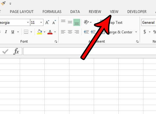
Step 2: Click the View tab at the top of the window.

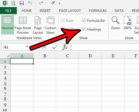
Step 3: Check the box to the left of Headings in the Show section of the ribbon. Your row labels should now be visible.

If you want to be able to quickly fill a row of numbers with consecutive numbers, then continue to the section below.
How to Fill Rows With Consecutive Numbers in Excel 2013
This section does not deal with the row labels that we added in the section below. Rather this is going to add values to your cells in the form of a numerical sequence that increases by one.
Following the steps in this section will allow you to do this quickly and error-free, which is likely a relief if you had previously done this by manually typing in all these values.
Step 1: Open your spreadsheet in Excel 2013.
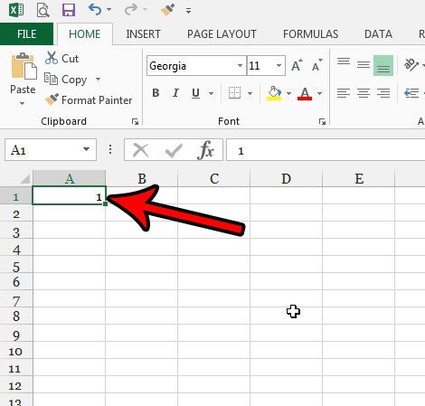
Step 2: Click in the top-most cell where you want to start the row numbering, then type the first number that you want to use for the numbering.

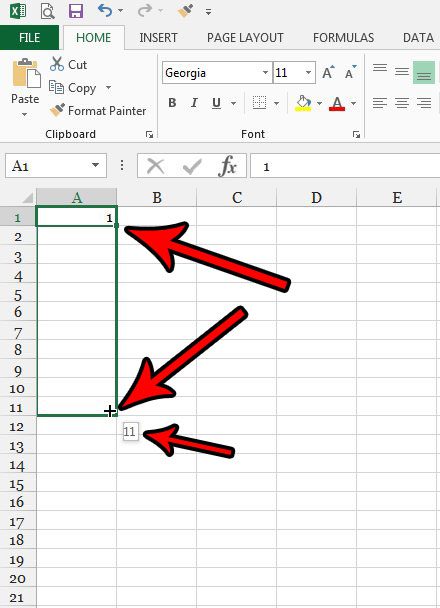
Step 3: Hold down the Ctrl key on your keyboard, click and hold on the bottom-right corner of the cell, then drag down until you have selected the number of cells to which you want to add the consecutive numbers.
Release the mouse button to fill those cells. Note that the number that goes into the bottom-most cell is shown as a small pop-up number slightly below your mouse cursor.

Now that you know how to add row numbering in Excel 2013, you can use these steps in the future whenever you have a spreadsheet that needs this type of formatting.
Do you have a large spreadsheet that is difficult to put into a summarized format without a lot of additional work? Find out more about pivot tables and see if that is a tool that can be useful for your Excel activity.

Matthew Burleigh has been writing tech tutorials since 2008. His writing has appeared on dozens of different websites and been read over 50 million times.
After receiving his Bachelor’s and Master’s degrees in Computer Science he spent several years working in IT management for small businesses. However, he now works full time writing content online and creating websites.
His main writing topics include iPhones, Microsoft Office, Google Apps, Android, and Photoshop, but he has also written about many other tech topics as well.