It’s really easy to miss some information when you are doing a lot of data entry in Microsoft Excel.
Sometimes you can just add that data at the bottom empty row in the spreadsheet, but you might need to know how to insert a row in Excel if the missed data needs to go in a specific spot.
Luckily there are a couple of different ways to accomplish this, which we will discuss in the guide below.
How to Add a New Row in Excel 2013
- Open your Excel file.
- Select the row number below where you want the new row.
- Click Home.
- Click the Insert arrow, then Insert Sheet Rows.
Our article continues below with additional information on how to insert a row in Excel, including pictures of these steps.
Would you like to print the top row of your worksheet on every page? Our repeat top row in Excel article can show you how.
Have you ever meticulously entered a lot of data into a spreadsheet, only to find that you need to add something between two existing rows?
You may have solved this issue by cutting all of your data and pasting it one row lower, or you might have even deleted a bunch of data to make room for the new row. But there are some options for adding rows in Excel that can make it much easier to include data within an existing dataset.
One of the most useful features of Microsoft Excel 2013 is how easy it is to manipulate and sort data. This is due largely to the grid-like structure of the worksheet, which consists of columns that run vertically throughout the sheet and rows that run horizontally. The rows and columns in your spreadsheet also have labels to identify them, which are indicated by row numbers and column letters.
This structure also makes it easy to add new rows or columns when you discover that you need to add more data in a location within your currently existing data. So check out our guide below to find out how you can insert a row into your Excel 2013 worksheet with just a few short steps.
Our Microsoft Excel add column guide provides ways that you can get totals for all of the values in a column, even after you’ve added more rows.
Adding a New Row Between Existing Rows in Excel 2013 (Guide with Pictures)
The tutorial below will show you how to insert a new row in the exact location of your worksheet where you want that row to appear. Any rows below the inserted row will simply be shifted down, and any formulas referencing a cell in those moved rows will automatically update to the new cell location.
Step 1: Open your worksheet in Excel 2013.
Step 2: Click the row below where you want your new row to be added.
For example, I want to add a row between what is currently row 4 and row 5, so I am selecting row 5. While I elect to select the entire row by clicking the row number, you can still insert the new row if you only select one of the cells in the row.
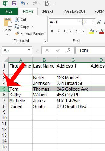
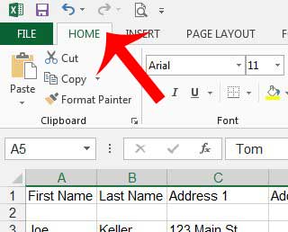
Step 3: Click the Home tab at the top of the window.
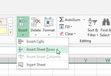
Step 4: Click the arrow under Insert in the Cells section of the navigational ribbon, then click Insert Sheet Rows.
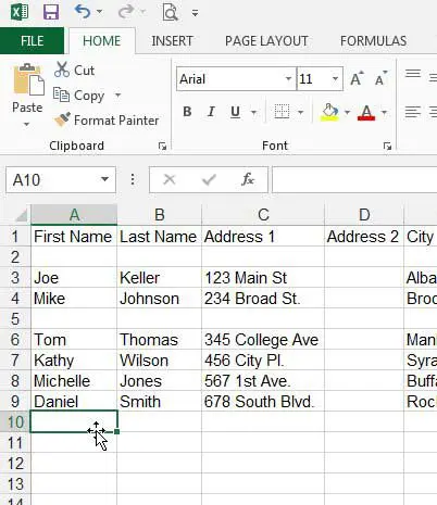
You should now have an empty row above the row that you had selected in Step 2, as in the image below.
Now that you know how to insert a row in Excel using the navigational ribbon, you might be wondering if there’s an alternate method for this process.
There is another way to insert a row in Excel, which we discuss below.
If you are editing your spreadsheet and find that some of the data needs to be merged, then read our guide on how to combine 3 columns in Excel.
Method 2 – How to Insert a Row in Excel 2013
Using options in the ribbon is helpful when you are performing a task that you don’t use very often. Typically the layout and organization in the ribbon makes sense, so you can usually find what you need.
But if you are performing an action with some frequency, then you might be looking for a faster way. Fortunately there is one for inserting rows in your spreadsheet.
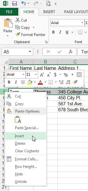
You can also insert a new row by right-clicking on the row number, then clicking the Insert option on the shortcut menu.
For additional information on adding rows to a spreadsheet, continue to the section below.
How to Insert Multiple Rows in Excel
While the options in our tutorial provide you solutions when you want to insert a single row, what if you need a bunch of them at once?
Fortunately you can use the same Insert button that we referenced above, but you need to select the number of rows that you want to insert first.
You can do this by clicking on a row number at the left side of the spreadsheet, then hold down the Shift key and click a lower row number to select all of the rows from that top one to the bottom one. For example, If I wanted to insert three rows I could click the row 2 heading, hold down Shift, then click the row 4 heading.
More Info on Inserting Excel Rows
While our article above was performed in Microsoft Excel 2013, these same steps are going to work for most other versions of Excel as well. For example, both of the options in this guide will work in Microsoft Excel for Office 365.
You can use a keyboard shortcut to insert a new row in Excel as well. Simply select the row number below where you want the new row, then press Ctrl + Shift + +. Note that the second plus in that shortcut indicates the “Plus” button that shares the = key on your keyboard. Using that shortcut to insert a row can be really handy, and it also makes it fairly easy to insert multiple rows quickly as well.
Taking advantage of the interaction between right clicking and row numbers provides you with some other ways to manage your data. For example, you can hide rows or delete rows by selecting a row number at the left side of the spreadsheet and choosing the desired action.
Any of the insertion methods that we describe in this article will apply to a row or column. So whether you are trying to insert rows or insert columns into your spreadsheet you will just need to work with the respective row numbers or column letters to make room for the range that you wish to add.
Do you have a row in your spreadsheet that you no longer need, or did you insert the new row in the wrong location? Learn how to delete a row in Excel 2013 when you have data that you want to remove.
Additional Sources

Matthew Burleigh has been writing tech tutorials since 2008. His writing has appeared on dozens of different websites and been read over 50 million times.
After receiving his Bachelor’s and Master’s degrees in Computer Science he spent several years working in IT management for small businesses. However, he now works full time writing content online and creating websites.
His main writing topics include iPhones, Microsoft Office, Google Apps, Android, and Photoshop, but he has also written about many other tech topics as well.