If you’ve worked on a big spreadsheet in Google Sheets and you needed to reference data in the first column, then you might have been frustrated with all of the scrolling.
Not only is this annoying and a waste of time, but it can also lead to mistakes.
Fortunately, you can freeze an entire column in your spreadsheet so that it remains locked to the left side of the window.
You can freeze columns in Google Sheets by selecting the column to freeze, selecting View, choosing Freeze, then clicking the option you want.
Google Spreadsheet Freeze Column Steps
- Open your spreadsheet.
- Select the column to freeze.
- Choose the View tab.
- Click Freeze.
- Choose the number of columns to freeze.
Our guide continues below with additional information about how to freeze Google Sheets columns, including pictures of these steps.
Making it easier to edit a document is a crucial component of any good productivity app.
Google Sheets has a variety of settings that can help you to accomplish this, including one feature that will let you “freeze” a row or a handful of columns on the left side of the sheet.
Once you choose to freeze some of your spreadsheet columns, they will stay fixed to the left side of the spreadsheet, even once you’ve scrolled to a point where they should be off-screen.
You can continue to the next section to learn more about using this setting.
Related: Learn how to make a header row in Google Sheets and make it easier to keep your data organized.
How to Make a Column Stay in Google Sheets
The steps in this article were performed in the desktop version of Google Sheets, but will also work in most other desktop or laptop Web browsers.
Step 1: Sign into Google Drive and open your spreadsheet.
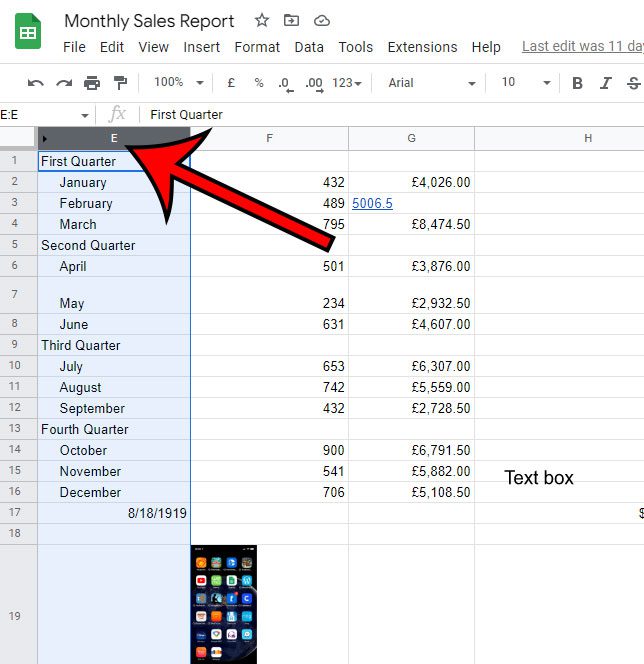
Step 2: Click the column letter at the top of the column you want to freeze.
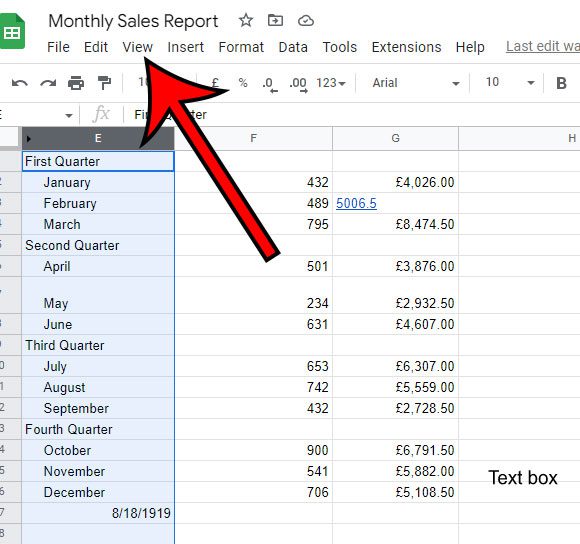
Step 3: Select the View tab at the top of the window.
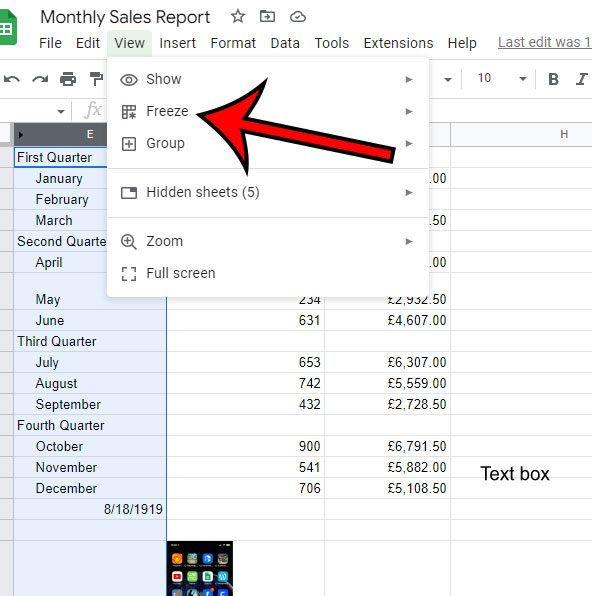
Step 4: Choose the Freeze option.
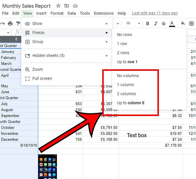
Step 5: Click 1 column, 2 columns, or the Up to column option.
Now that you know how to freeze columns in Google Sheets, you can use this method anytime that you have a column of data that you want to remain visible as you edit your data.
If you want to unfreeze a column in Google Sheets, then you can go back to the View > Freeze menu and select the No columns option.
What Does it Mean to Freeze Columns?
In a spreadsheet, freezing columns refers to the ability to keep certain columns displayed while scrolling through the rest of the data. When you freeze columns, you ensure that the important information in your spreadsheet is always displayed, even if you scroll to the right or bottom of the page. This makes referencing essential information and comparing data across columns easy.
Most spreadsheet systems, including Microsoft Excel and Google Sheets, allow you to freeze columns. To freeze columns, simply choose the column or columns to be frozen, then go to the “View” menu and select “Freeze.” You can then choose to freeze the first column, the first row, or a certain number of columns.
You will be able to see the frozen columns once you have frozen them in your spreadsheet.
Why Would I Want to Freeze Columns in a Spreadsheet?
For a variety of reasons, freezing columns in a spreadsheet can be extremely handy. The following are some of the primary advantages of freezing columns in a spreadsheet:
Simple access – By freezing columns, you can keep key information visible while scrolling through the rest of the data in the spreadsheet. This is especially beneficial if you are working with a large spreadsheet and need to refer to crucial information at all times.
Improved organization – By freezing columns, you can better organize your spreadsheet by ensuring that the most critical information is always visible. This can help you compare data across columns and quickly discover the information you require.
Improved readability – By freezing columns, you can ensure that your spreadsheet’s critical information is always in the same position, making it easier to read and interpret the data. This is especially beneficial if you are dealing with a complex spreadsheet and need to retrieve information quickly.
Increased productivity – You may save time and increase your productivity by keeping vital information visible at all times. Instead of repeatedly scrolling back to the top of the spreadsheet to find important information, you can simply keep it visible as you work.
Improved collaboration – When working on a spreadsheet with a group, freezing columns might make it easier for everyone to obtain the information they require. This can aid in the reduction of confusion and the improvement of collaboration.
Customizable – You can select to freeze any number of columns in your spreadsheet and unfreeze them at any moment. This means you may tailor your spreadsheet to your specific requirements and update it as those requirements change.
Improved data analysis – By freezing columns, you may compare data across columns more quickly and do more accurate data analysis. This is especially handy when dealing with enormous datasets and needing to quickly find trends and patterns in the data.
Better presentation – When presenting a spreadsheet to others, freezing columns can help make the data more legible and understandable. You may ensure that your presentation is clear and effective by putting vital information in the same area.
Finally, freezing columns in a spreadsheet can be an extremely valuable tool for a variety of applications. Whether you’re working with a huge spreadsheet, collaborating with a team, or simply want to improve the readability of your data, freezing columns can help.
More Information on Freezing Google Sheets Columns
When you freeze columns in Google Sheets, you can keep specific columns displayed while scrolling through the rest of the data. This is useful if you have a huge spreadsheet and want to ensure that specific columns remain visible no matter how far down the page you scroll. This might help you remember critical information or keep a vital column visible while looking at other columns.
To freeze columns in Google Sheets, first choose the column or columns you want to freeze. You can pick several columns by clicking and dragging on the letter that symbolizes the column at the top of the sheet. After you’ve chosen the columns you wish to freeze, go to the “View” menu and pick “Freeze.” In Google Sheets, there are numerous choices for freezing columns, including freezing the first column, the top row, or a certain number of columns.
When you freeze columns in Google Sheets, you will be able to see them even when you scroll to the right. This enables comparing data across columns and referencing crucial information easier. If you wish to keep numerous columns displayed when scrolling, you can freeze them. If you have numerous key columns that you wish to refer to while looking at other data, this can be handy.
It is vital to understand that freezing columns in Google Sheets is not the same as hiding columns. Columns that are frozen remain visible while scrolling, whereas columns that are hidden are completely removed from view. You can freeze columns in Google Sheets even if other columns in the sheet are hidden.
In Google Sheets, go to the “View” menu and select “Freeze” to unfreeze columns. You can then select “No frozen” to unfreeze any presently frozen columns. This allows you to browse through all of the columns in the sheet easily.
Finally, freezing columns in Google Sheets is a handy tool that lets you keep critical columns visible while scrolling through a huge spreadsheet. You can freeze one or more columns at a time and unfreeze them at any time. Freezing columns in Google Sheets is a simple and effective option if you are dealing with a huge spreadsheet or simply want to ensure you can reference vital information while looking at other data.

Matthew Burleigh has been writing tech tutorials since 2008. His writing has appeared on dozens of different websites and been read over 50 million times.
After receiving his Bachelor’s and Master’s degrees in Computer Science he spent several years working in IT management for small businesses. However, he now works full time writing content online and creating websites.
His main writing topics include iPhones, Microsoft Office, Google Apps, Android, and Photoshop, but he has also written about many other tech topics as well.


