How to Make a Row Float in Google Sheets

Google Sheets has a lot of options that can make it easier for you to enter and organize data.

Some of these options don’t involve any formulas or data tolls, however, and will affect the display of the rows and columns in your spreadsheet.

One option that is particularly noteworthy involves “floating” a row so that it stays locked at the top of the screen while you are scrolling down, past the point where that row would be naturally visible.

You can make a row float in Google Sheets by selecting the bottom row to float, clicking View, then Freeze, then Up to row x.

How to Freeze a Google Sheets Row

1. Open your spreadsheet.
2. Select the row number to freeze.
3. Click View.
4. Choose Freeze.
5. Select Up to row.

Our guide continues below with additional information on how to make a row float in Google Sheets, including pictures of these steps.

Have you ever worked on a spreadsheet in Google Sheets that someone else created, and you discovered that the top row seemed to be floating?

This becomes noticeable when you scroll down but are still able to see the header row that contains descriptions of the data contained in each column.

At first, this might seem strange or potentially problematic, but it can actually be really helpful because you don’t need to remember what kind of data goes into each column.

If you like this option and want to start using it, then you can continue to the next section to see how to create floating rows in Google spreadsheets.

Related: This Google Sheets tutorial will show you how to create a header row so that you can make the data in your spreadsheet easier to identify.

How to Create a Floating Google Sheet Row

The steps in this section were performed in the desktop version of Google Chrome. These steps will also work in other laptop and desktop Web browsers like Mozilla Firefox and Microsoft Edge.

Step 1: Sign into your Google Drive and open your spreadsheet.

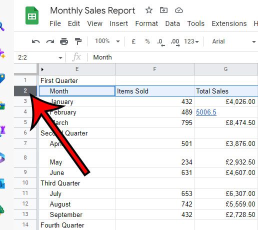
Step 2: Click the row number at the left side of the spreadsheet for the bottom row that you wish to float.

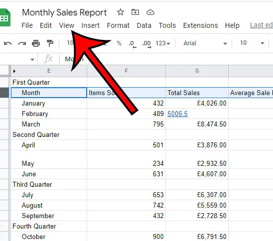
Step 3: Select the View tab in the menu bar at the top of the window.

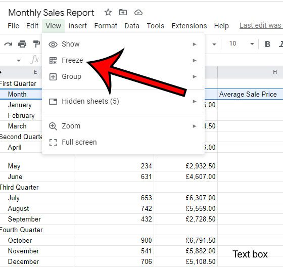
Step 4: Choose the Freeze option from the dropdown menu.

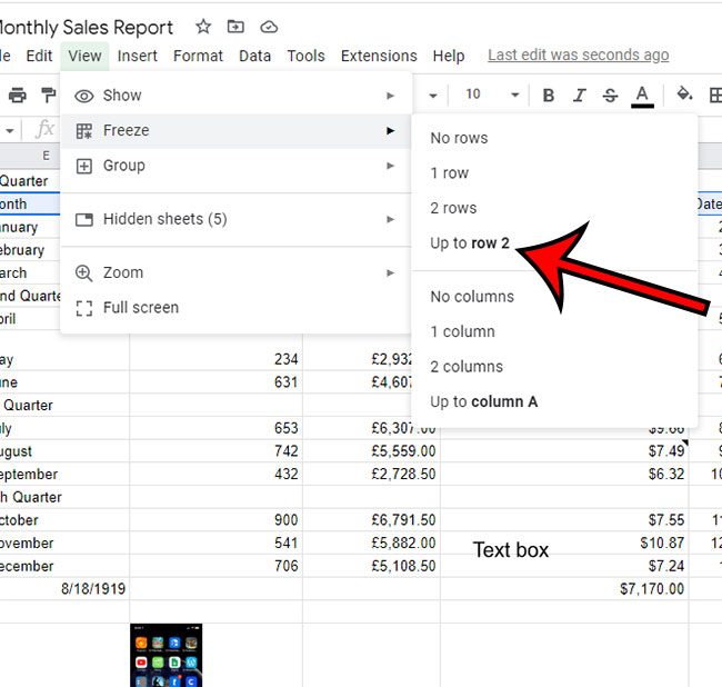
Step 5: Click the Up to row x option, where x is the number of the row that you selected.

Note that you can also choose to float No rows, 1 row, or 2 rows from this menu as well.

Now that you know how to make a row float in Google Sheets, you will be able to use this feature for any spreadsheet that is getting tough to edit because there are too many rows of data to fit on one screen.

More Information About Floating or Freezing Rows in Google Spreadsheets

One other option that you have for freezing rows involves a dragging shortcut.

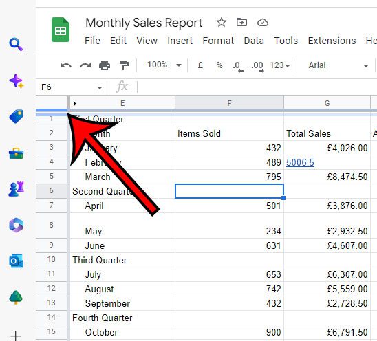
You can make a row float in Google Sheets by dragging the bottom border of the empty gray box above row 1, then releasing your mouse once that border is below the bottom row that you want to float.

If you want to stop floating a row, then you can either go back to View > Freeze > and select the No rows option, or you can click and drag the bottom border back to the gray rectangle.

Note that this method for floating a row will only affect the current spreadsheet. This setting won’t be applied automatically to other spreadsheets, so you will need to make this adjustment for any other file where you want to use this option.

For many spreadsheets, you will almost certainly only want to freeze the first row.

When you freeze rows in a spreadsheet, make sure they stay visible when you scroll so you don’t enter data into the wrong column.

However, if your spreadsheet structure demands several columns or if you use more than one row to represent significant information, you may wish to freeze more than one row. If this is the case, you can opt to freeze rows up until the one currently chosen in your spreadsheet.

To choose a row, click the row number on the left side of the window. The same action can be used to pick a full column by clicking the column letter at the top of the sheet.

The View menu at the top of the window not only allows you to freeze rows but also allows you to hide or reveal gridlines, view formulas, and zoom in on your data.

While it lacks the variety of viewing choices provided in Microsoft Excel, many Excel users have considered Google Sheets to be a competent alternative to Microsoft’s premium spreadsheet application.

As a previous Excel user, transitioning to Google Sheets can be difficult.

While many of the application’s functions are easy to find, others, particularly the printing and viewing options, may require some practice until you become acquainted with them.

If there is something you wish to modify about the way your Google Sheet appears on the screen or when you print, there is most likely a way to do it.

Familiarize yourself with the View menu and the File > Print menu, as that is where the majority of those options can be located.