To hide a column in Google Sheets, right-click the column letter and choose Hide column. Arrows appear where the column was. Click either arrow to show it again. You can also press Ctrl + Alt + 0 (Command + Option + 0 on a Mac) to hide the selected columns. To group columns so you can collapse them with a button, use View > Group.
These steps come from Google’s Freeze, group, hide, or merge rows & columns help page (computer and iPhone/iPad versions) and its Keyboard shortcuts for Google Sheets list.
How to Hide a Column in Google Sheets
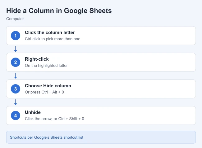
- Click the column letter. To select more than one, hold Ctrl (Command on a Mac) and click the others.
- Right-click the selection.
- Choose Hide column.
Result: the column disappears and Google says an arrow appears over the spot where it was. With several rows or columns selected, the menu option names the range, such as Hide rows 5 – 7.
How to Unhide a Column
- Click an arrow. Google says to click the arrow where the column letter used to be.
- Use the shortcut. Try selecting the columns on both sides of the hidden ones and pressing Ctrl + Shift + 0 (Command + Shift + 0 on a Mac).
Excel handles this differently, so if you also work there, see how to unhide all rows in Excel.
How to Group or Ungroup Columns
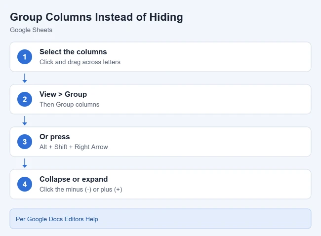
- Select the columns.
- Click View > Group.
- Choose Group columns or Ungroup columns.
Result: a bracket appears above the columns. Google says to click Minus (-) to collapse the group and Plus (+) to expand it.
Try grouping for anything readers should be able to open, like monthly detail under a quarterly total, and hiding for things nobody needs to see.
Keyboard Shortcuts
From Google’s shortcut list (Windows; on a Mac, use Command for Ctrl and Option for Alt):
- Hide column: Ctrl + Alt + 0
- Unhide column: Ctrl + Shift + 0
- Hide row: Ctrl + Alt + 9
- Unhide row: Ctrl + Shift + 9
- Group: Alt + Shift + Right Arrow; ungroup: Alt + Shift + Left Arrow
- Collapse a group: Alt + Shift + Up Arrow; expand: Alt + Shift + Down Arrow
How to Hide a Column in the Sheets App
- Open the spreadsheet in the Google Sheets app.
- Tap the column letter.
- In the menu that appears, tap the right arrow, then Hide column.
Google says grouping works the same way in the app: highlight the columns, tap them, tap the right arrow, and choose Group.
Things to Know About Hidden Columns
- Formulas still count them. SUM includes hidden rows. To total only visible rows, it suggests SUBTOTAL with codes 101 to 111, such as =SUBTOTAL(109, B2:B20).
- Hiding isn’t security. Anyone who can edit the sheet can unhide columns, and hidden data comes along in downloads and copies. Use protected ranges to stop edits. To unlock them later, see how to remove protection from a sheet or range in Google Sheets.
- Whole tabs: right-click a sheet tab and choose Hide sheet. Bring it back with View > Hidden sheets.
Frequently Asked Questions
Why can’t I see the arrows to unhide?
The small arrows are the only sign columns are hidden, so they’re easy to miss. Look for a skipped letter in the column headings, or use the unhide shortcut. If you also use Excel in a browser, see how to hide columns in Excel Online.
Can people I share the sheet with see hidden columns?
They won’t see them at first, but editors can unhide them, and the data is still in the file. Don’t rely on hiding to keep information private.
Related Guides
- How to freeze columns in Google Sheets
- How to rename, add, or hide sheet tabs
- How to merge cells in Google Sheets

Matthew Burleigh is the founder, head writer, and editor of Solve Your Tech, which he launched in 2012. He has written technology tutorials since 2008 and worked in IT since 2003, including small-business support, IT management, and consulting. He holds Bachelor’s and Master’s degrees in Computer Science from Arizona State University.
Matthew writes practical guides for Windows, iPhone and iPad, Microsoft Office, Outlook, Google apps, and Android. Solve Your Tech’s guides are tested on current devices or checked against official product documentation, with clear steps, sources, and update dates.
Read more about Matthew and how Solve Your Tech writes and updates its guides, or report a correction.