To insert an arrow in Excel, go to the Insert tab, select Shapes, and choose Line Arrow under Lines. Then click and drag on the worksheet to draw it, and hold Shift while you drag to keep the arrow straight.
These steps work in Excel for Microsoft 365, Excel 2024, 2021, 2019 and 2016 on Windows, and the same Insert > Shapes path is in Excel 2013. Mac menus are close to the same; Mac keyboard differences are noted where they matter.
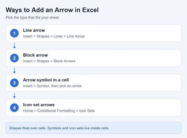
Which Kind of Arrow Do You Need?
Excel has two very different kinds of arrows, and picking the right one first saves time.
| You want to | Use | Where it lives |
|---|---|---|
| Point at a cell, chart or note | Line arrow or block arrow shape | Floats above the cells |
| Link boxes in a flowchart | Connector arrow | Floats, stays attached to the boxes |
| Put an arrow next to a number | Symbol, Alt code or UNICHAR formula | Inside the cell as text |
| Show up or down trends automatically | Icon sets or a custom number format | Inside the cell, driven by the value |
A shape is a drawing, so it doesn’t sort, filter or move with your data the way cell contents do. A symbol is a text character, so it can sit in a cell, be copied down a column and appear in formulas.
How to Insert an Arrow Shape in Excel
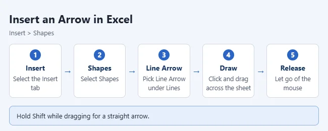
- Select the Insert tab.
- In the Illustrations group, select Shapes. A gallery of shapes opens.
- Under Lines, select Line Arrow. Rest your pointer on each style to see its name before you click.
- Click where you want the arrow to start, hold, and drag to where you want it to point.
- Release the mouse button. The arrow appears with a small circle at each end, and the Shape Format tab opens on the ribbon.
The arrowhead goes at the end where you finished dragging. To point the other way, drag the end handles, or change the arrowhead style as shown below. Holding Shift while you drag locks the line to straight horizontal, vertical or 45 degree angles.
Want a thick, filled arrow instead? Pick one from the Block Arrows section of the Shapes menu and drag to draw it. Block arrows have a fill color, so you can type text inside them: right-click the arrow and choose Edit Text.
To draw several arrows in a row, right-click the arrow style under Lines and choose Lock Drawing Mode. Draw as many as you need, then press Esc when you’re done. Microsoft covers drawing and Lock Drawing Mode in Draw or delete a line or connector.
Making the same diagram for a presentation? Here is how to add an arrow in Google Slides.
Draw a Line Without an Arrow in Excel
For a plain line, choose Insert > Shapes > Line rather than Line Arrow. Click the starting point on the worksheet and drag to the ending point, holding Shift for a straight horizontal or vertical line. Select the line and use Shape Format > Shape Outline to adjust its color, weight or dashes. A drawn line floats over the cells, so use a cell border instead when the line should follow a row or column. You can make a thicker bottom border in Excel for that.
How to Connect Two Shapes With an Arrow
If you’re building a simple flowchart, use a connector instead of a plain line. A connector stays attached to the shapes and moves with them.
- Go to Insert > Shapes and pick a connector arrow under Lines (straight, elbow or curved).
- Rest your pointer on the first shape until gray connection dots appear on its border.
- Click a dot and drag to a connection dot on the second shape. Both ends turn into small attached handles.
- Drag one of the shapes. The arrow bends and follows it.
The last three styles under Lines (Curve, Freeform Shape and Scribble) aren’t connectors. If no dots appear, you picked a style that isn’t a connector.
For a ready-made process diagram with arrows already in place, try Insert > SmartArt and pick a layout from the Process category. You type your steps in the text pane and Excel draws the boxes and arrows for you.
How to Change the Arrow’s Color, Weight and Arrowhead
Select the arrow first. If you don’t see the Shape Format tab, make sure the line is selected; you might need to double-click it.
- Color: Shape Format > Shape Outline, then pick a color. Use More Outline Colors for a custom color.
- Thickness: Shape Outline > Weight, then pick a weight. Choose More Lines for a custom weight.
- Dashed line: Shape Outline > Dashes.
- Arrowhead style: Shape Outline > Arrows, then pick a style. This menu also has double-headed styles for a two-way arrow. More Arrows opens the Format Shape pane, where you can set the begin and end arrow type and size separately. To remove the arrowheads, choose Arrow Style 1.
- Quick Styles: pick a predefined style on the Shape Format tab for a fast makeover.
For block arrows, use Shape Fill for the inside color and Shape Outline for the border. To change several arrows at once, select the first one, then hold Ctrl and select the others. All of these options are on Microsoft’s Change the color, style, or weight of a line page.
How to Move, Rotate, Copy or Delete an Arrow
- Move it: click the arrow and drag it. Drag either end to change its length or direction.
- Rotate a block arrow: drag the curved rotation handle above it, or use Shape Format > Rotate for exact 90 degree turns and flips.
- Copy it: select the arrow, press Ctrl+C, then Ctrl+V. Holding Ctrl while you drag also makes a copy.
- Delete it: click the arrow and press Delete. To delete several, hold Ctrl while you select them, then press Delete.
How to Put an Arrow Inside a Cell
Shapes float above the cells rather than being part of a cell’s contents. To put an arrow in a cell as text, use one of the methods below. Each one gives you a character you can resize, bold or color with the normal font tools on the Home tab.
Use the Symbol Window
- Click the cell.
- Go to Insert > Symbol. The Symbol window opens.
- Leave Font set to (normal text) and pick Arrows in the Subset list. Not every font has this subset.
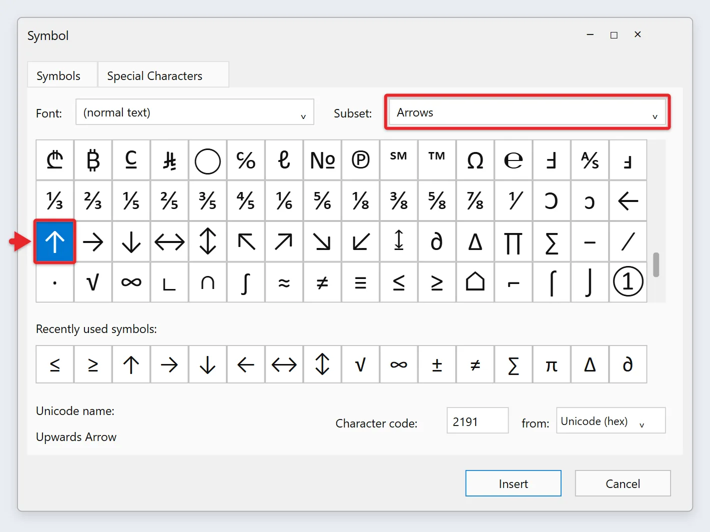
- Select an arrow, select Insert, then select Close. The arrow appears in the cell.
You can also type a code in the Character code box with from set to Unicode (hex): 2190 is left, 2191 is up, 2192 is right and 2193 is down. Microsoft’s Insert a symbol page covers the Symbol window and applies to Excel too. The same window adds bullet points, so you can put a bulleted list in an Excel cell.
Type an Alt Code on Windows
On a keyboard with a number pad, turn on Num Lock, double-click the cell, hold Alt and type the number on the number pad, then let go of Alt:
| Arrow | Alt code | Unicode number for UNICHAR |
|---|---|---|
| ↑ | Alt+24 | 8593 |
| ↓ | Alt+25 | 8595 |
| → | Alt+26 | 8594 |
| ← | Alt+27 | 8592 |
| ↔ | Alt+29 | 8596 |
| ▲ | Alt+30 | 9650 |
| ▼ | Alt+31 | 9660 |
The number keys above the letters won’t work for Alt codes. On a laptop without a number pad, use the Symbol window or the emoji panel instead.
Use the Windows Emoji Panel or the Mac Character Viewer
On Windows 11, double-click the cell, press Windows key + period, select Symbols in the panel that opens, and pick an arrow (more shortcuts are in Microsoft’s Windows keyboard tips). On a Mac, press Fn/Globe+E or choose Edit > Emoji & Symbols, search for “arrow” and click one, as shown in Apple’s Mac emoji and symbols guide.
Use the UNICHAR Formula
Type =UNICHAR(8593) in a cell to show an up arrow. Swap in the numbers from the table above for other directions. Microsoft’s UNICHAR function page lists Excel for Microsoft 365, 2024, 2021, 2019 and 2016; the function first appeared in Excel 2013. The older CHAR function stops at 255, so it can’t return these arrows.
How to Show Up and Down Arrows Based on Your Numbers
Picking arrows by hand gets tedious for a long column. These three methods choose the arrow for you.
Icon Sets
- Select the cells with your numbers.
- On the Home tab, select Conditional Formatting.
- Point to Icon Sets and choose one of the arrow sets, such as 3 Arrows (Colored). Each cell gets a green up, yellow sideways or red down arrow.
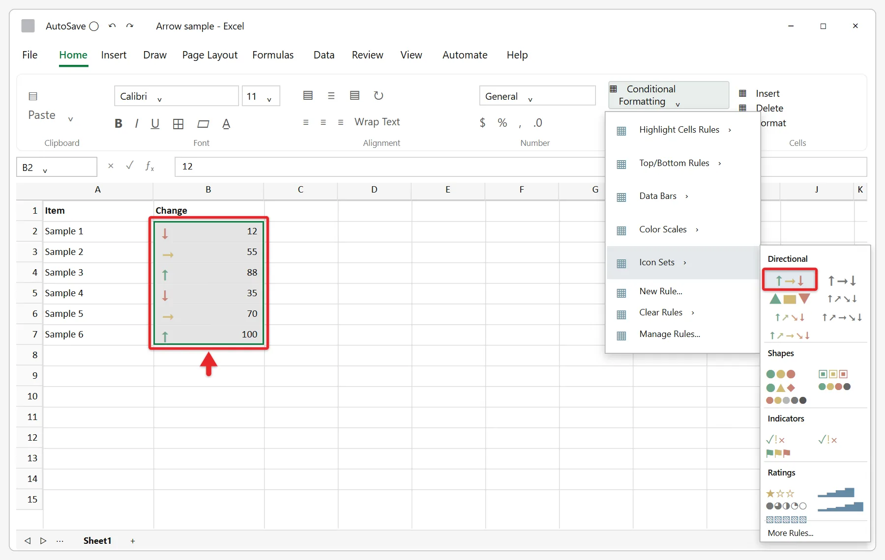
Microsoft’s icon set guide explains that icon sets sort values into three to five groups by threshold. Its three-icon example uses one icon for values at or above 67 percent, another for 33 to 67 percent, and a third for values below 33 percent. That means a small gain can still get a yellow or red arrow when it falls in the bottom third of the range.
To set your own cutoffs, go to Conditional Formatting > Manage Rules, select the rule and choose Edit Rule. Change Type from Percent to Number and enter values, for example green when the value is greater than 0. Check Show Icon Only to hide the numbers, or Reverse Icon Order to flip the colors. Icon sets work best on a column of changes, such as this month minus last month, rather than on raw totals.
An IF Formula
If C2 holds the change, =IF(C2>0,UNICHAR(8593),IF(C2<0,UNICHAR(8595),UNICHAR(8594))) shows up, down or sideways. Copy it down the column, and each row picks its own arrow. Because the result is text, you can color it with conditional formatting.
A Custom Number Format
This keeps the cell a real number while showing an arrow in front of it.
- Select the cells and press Ctrl+1 to open Format Cells.
- On the Number tab, choose Custom.
- In the Type box, enter
[Green]"▲ "0;[Red]"▼ "0;"→ "0and select OK.
Positive numbers show a green up arrow, negative numbers a red down arrow, and zero a sideways arrow. The minus sign is hidden because the second section has none, though the value is still negative in formulas. Microsoft’s number format guidelines explain the positive, negative and zero sections and the color names.
Other Ways to Add Arrows
- Icons: in Excel for Microsoft 365, go to Insert > Icons, search for “arrow,” select one and choose Insert. Icons resize without blurring, and you can recolor one by right-clicking it and choosing Fill, per Microsoft’s Insert icons page. If your version has Place in Cell for pictures, the same idea lets a graphic sit inside a cell. Follow the steps to insert a picture into a cell in Excel.
- Arrow on a line chart: right-click the line, choose Format Data Series, open Fill & Line, and pick an End Arrow type. Column charts don’t have this option, so draw an up arrow shape from Block Arrows on top of the column instead.
- Text box next to an arrow: to label an arrow with a value that updates, display a formula result in a text box.
When the Shapes Button Is Grayed Out
- The Shapes button is grayed out: the sheet may be protected. Go to Review > Unprotect Sheet, or you may be editing a cell; press Enter or Esc first.
- The arrow moved or stretched when I resized columns: right-click the arrow, choose Format Shape (or Size and Properties), and under Properties choose Don’t move or size with cells.
- A box shows instead of the arrow: the cell’s font doesn’t have that character. Switch the cell to Calibri, Arial or Segoe UI Symbol.
- Alt codes type nothing or the wrong thing: turn on Num Lock and use the number pad, not the top row.
- The arrow isn’t straight: drag an end handle again while holding Shift.
Excel Arrow Questions
How do I make the arrow perfectly straight?
Hold Shift while you drag to draw it. Shift keeps the line at horizontal, vertical or 45 degree angles.
How do I make a two-way arrow?
Select the arrow, then go to Shape Format > Shape Outline > Arrows and pick a style with a head on both ends. For text, use the ↔ symbol (Alt+29 or UNICHAR 8596).
Why can’t I see the Shape Format tab?
The arrow isn’t selected. Click it, or double-click it.
Can an arrow move with my data when I sort?
A shape doesn’t sort with rows. Use a symbol, formula or icon set inside the cell when the arrow belongs to a row of data.
What’s the difference between an arrow shape and an arrow symbol?
A shape floats above the worksheet and can point anywhere. A symbol or icon set sits inside a cell as part of your data. For marking up an image rather than a spreadsheet, draw a straight line in Photoshop instead.
Next, you can color the cells in Excel that your arrows point to, or add a column in Excel to make room for a new column of trend arrows.

Matthew Burleigh is the founder, head writer, and editor of Solve Your Tech, which he launched in 2012. He has written technology tutorials since 2008 and worked in IT since 2003, including small-business support, IT management, and consulting. He holds Bachelor’s and Master’s degrees in Computer Science from Arizona State University.
Matthew writes practical guides for Windows, iPhone and iPad, Microsoft Office, Outlook, Google apps, and Android. Solve Your Tech’s guides are checked step by step against the device or app maker’s own documentation and tested on his own devices whenever he has the hardware or software, with clear steps, sources, and update dates.
Read more about Matthew and how Solve Your Tech writes and updates its guides, or report a correction.