How to Subtract in Excel (Cells, Columns, Dates and Percentages)

To subtract in Excel, click an empty cell, type an equal sign, then the first cell, a minus sign and the second cell, such as =A2-B2, and press Enter. Excel has no SUBTRACT function, so every subtraction uses the minus sign, sometimes together with SUM. This guide covers Excel for Microsoft 365, Excel 2024, 2021, 2019 and 2016 on Windows and Mac, plus Excel for the web. The same formulas work in older versions such as Excel 2010 and 2013.

The steps follow Microsoft’s Subtract numbers in Excel and Add and subtract numbers articles.

Which Subtraction Method Should You Use?

What you want	Use this	Example
One number minus another	Minus sign with cell references	=A2-B2
One number minus several cells	Minus sign and SUM	=A2-SUM(B2:B6)
Column A minus column B, row by row	One formula, filled down	=A2-B2, then drag the fill handle
The same number taken off every row	Absolute reference	=A2-$E$1
Change the numbers in place, no formula	Paste Special > Subtract	Copy the number, then Ctrl+Alt+V
A percentage off a price	Multiply by 1 minus the percentage	=B2*(1-20%)
Days or hours between two values	End minus start	=B2-A2

How to Subtract Two Cells in Excel

Using cell references instead of typed numbers is the better habit, because the answer updates on its own when you change either value.

1. Type your first number in one cell (for example, 150 in A2) and the number to take away in another (for example, 45 in B2).
2. Click the empty cell where you want the answer, such as C2.
3. Type = to start the formula.
4. Click cell A2, type a minus sign -, and then click cell B2. The formula bar now shows =A2-B2.
5. Press Enter (or Return on a Mac). The cell shows 105.

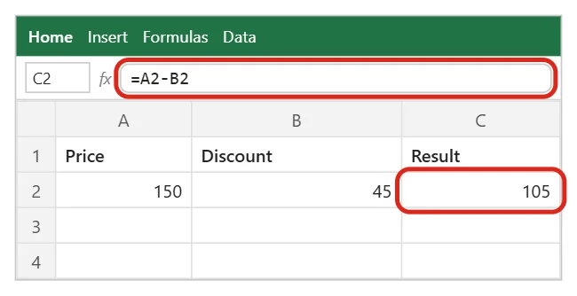
The cell displays the result, but the formula is still there. Click the cell and look at the formula bar to see it. You can also subtract typed numbers directly, such as =150-45, but that answer won’t change if your data does.

Subtract Several Numbers From One Cell

To take more than one value away from a starting number, keep adding minus signs: =A2-B2-C2-D2. Excel works from left to right, so =50-10-5-3 returns 32.

For a longer list, add up everything you want to take away with SUM and subtract the total in one step. If your income is in B1 and your expenses are in B2 through B6, use =B1-SUM(B2:B6). This is easier to read and keeps working if you insert a new expense row inside the range. Need the total on its own first? See how to sum a column in Excel.

If your list already holds negative numbers for the amounts to take away, SUM alone does the subtraction. Microsoft’s example, =SUM(100,-32,15,-6), returns 77.

Subtract One Column From Another

This is the most common real task: revenue minus cost, budget minus actual, or this year minus last year on every row.

1. In the first row of an empty column, type the formula for that row, such as =B2-C2, and press Enter.
2. Click the cell again and point at the small square in its bottom-right corner (the fill handle).
3. Drag the fill handle down to the last row of data, or double-click it to fill down to the end of the data automatically.

Excel adjusts the row number in each copy, so row 3 becomes =B3-C3, row 4 becomes =B4-C4, and so on.

In Excel for Microsoft 365 you can also subtract whole ranges in one formula, such as =B2:B11-C2:C11. The answers spill into the cells below. If anything is already in those cells, you’ll see a #SPILL! error until you clear them, as Microsoft explains in its dynamic array guide.

Subtract the Same Number From a Whole Column

To take one fixed value away from every row, such as a $25 discount stored in cell E1, lock that cell with dollar signs so it doesn’t move when you fill the formula down.

1. In C2, type =B2-$E$1 and press Enter.
2. Drag the fill handle down the column.
3. Check a lower row. It should read =B5-$E$1: the B reference changed, but $E$1 stayed fixed.

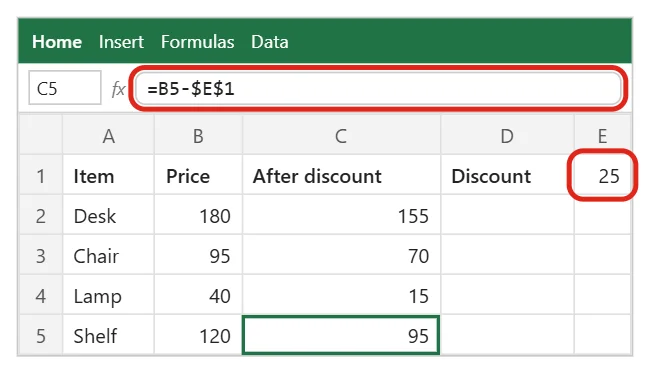
You don’t need to type the dollar signs. Click the reference in the formula bar and press F4 to switch it to an absolute reference. If you forget to lock it, the copies point to E2, E3 and so on, which are usually empty, so the formula subtracts nothing and the numbers look unchanged. For a typed number, =B2-25 works too, but storing it in a cell makes it easy to change later.

Subtract Without a Formula Using Paste Special

Paste Special can take a number away from a block of cells and leave plain values behind, with no extra column.

Warning: this permanently replaces the original values in the selected cells. Copy the column somewhere safe first if you might need the old numbers, and press Ctrl+Z right away if the result isn’t what you wanted.

1. Type the number to subtract in an empty cell, such as 10, and copy that cell with Ctrl+C.
2. Select the cells you want to reduce.
3. Press Ctrl+Alt+V, or go to Home > Paste > Paste Special.
4. Under Operation, select Subtract, then click OK.
5. Delete the helper number you typed in step 1.

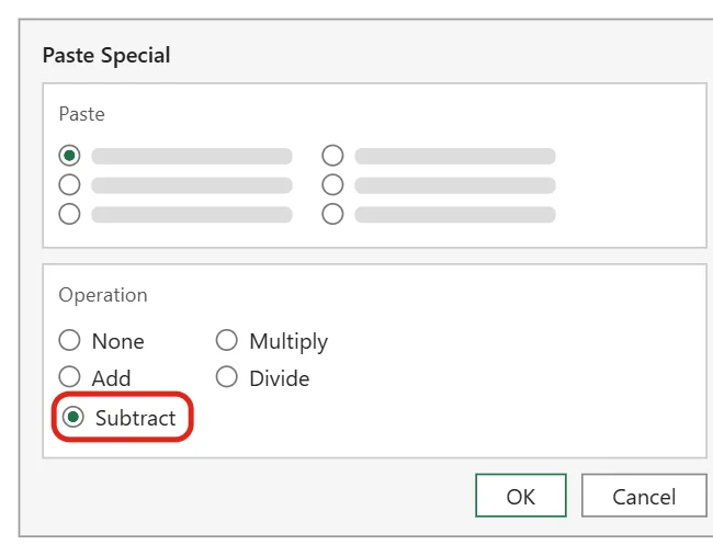
Microsoft describes the Subtract option as taking the copied data away from the data in the destination cells (Paste options). If you copy a range instead of one cell, each copied value is subtracted from the matching destination cell.

Subtract a Percentage From a Number

A plain =B2-20% subtracts 0.2, not 20 percent of B2. To take 20% off a price in B2, multiply by what is left instead: =B2*(1-20%), or =B2*(1-C2) with the percentage in C2. A $50 price becomes $40.

Subtracting one percentage from another, such as =C2-B2 with 35% and 28%, gives the change in percentage points (7%), not the percent change. The percentage formula guide covers increases, decreases and percent change in more detail.

Subtract Dates and Times

Excel stores dates as serial numbers, so =B2-A2 with an end date in B2 and a start date in A2 returns the number of days between them. If the answer looks like a date, select the cell and choose General on the Home tab. To count weekdays only, use =NETWORKDAYS(A2,B2). For ages, months and years, see how to subtract dates and calculate age in Excel.

Times work the same way. =B2-A2 with 9:00 AM and 5:30 PM returns 8:30 when the cell is formatted as time. To turn the result into a number of hours, multiply by 24: =(B2-A2)*24 returns 8.5. Multiply by 1440 for minutes. For totals over 24 hours, apply the custom format [h]:mm (press Ctrl+1, then Custom).

If a date or time subtraction comes out negative, Excel shows ##### instead of a value, because dates and times can’t be below zero. Check that the later value comes first in the formula.

Subtract Values on Different Sheets

Put the sheet name and an exclamation point in front of the cell: =Sheet1!B2-Sheet2!B2. If a sheet name contains spaces or symbols, wrap it in single quotes, such as ='Sales 2026'!B2-'Sales 2025'!B2. The easiest way is to type =, click the cell on the first sheet, type -, then click the other sheet’s tab and the cell, and press Enter.

How to Check Your Subtraction Formulas

Press Ctrl+` (the grave accent key, usually left of 1) to switch between showing results and showing formulas, or click Show Formulas on the Formulas tab. Scan down the column to make sure each row points to the right cells and that locked references kept their dollar signs. Press the same shortcut again to go back.

Troubleshooting Subtraction in Excel

• The formula shows as text instead of an answer. The formula is missing its leading =, or the cell was formatted as Text before you typed. Change the format to General, click in the formula bar and press Enter.
• You get #VALUE!. One of the cells holds text, such as a number with a space or the word “n/a”. Fix or clear that cell.
• The answer is wrong but there is no error. A number may be stored as text (it often sits on the left side of the cell with a small green triangle). Select it, click the warning icon and choose Convert to Number. Blank cells count as zero.
• You see a date instead of a number. Excel copied a date format from a nearby cell. Select the result and choose General on the Home tab.
• You see #####. The column is too narrow, or a date or time result is negative. Widen the column, or swap the order of the values.
• Results don’t change when you edit the numbers. The workbook may be set to manual calculation. Go to Formulas > Calculation Options and choose Automatic.

Frequently Asked Questions

Next Step

Start with =A2-B2 for a single difference, then fill it down or lock a cell with F4 when you need the same subtraction on every row. To make negative results stand out, try conditional formatting in Excel.