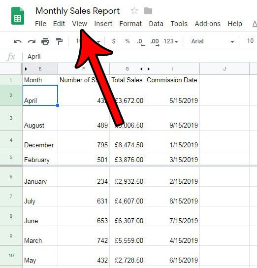
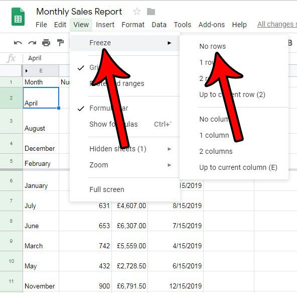
You can unfreeze a row in Google Sheets by selecting the View tab at the top of the window, choosing Freeze, then clicking No Rows.
Many of the issues that you might encounter when working with a spreadsheet may not actually have anything to do with the data in your cells. After you’ve gone through the trouble of generating your data and created all your formulas and charts, you may find that you’re having trouble simply navigating through all of that data.
One way to resolve this issue is by freezing a row or two at the top of the sheet. This lets you scroll down while still keeping important data, such as your row headings, visible. But if you’re working on a sheet that was created by someone else and it has these frozen rows, then you may be looking for a way to unfreeze them. Our guide below will show you how.
How to Unfreeze Rows in Google Sheets
The steps in this article were performed in the desktop version of the Google Chrome Web browser, but will also work in other desktop browsers like Edge and Firefox.
Step 1: Sign into your Google Drive at https://drive.google.com and open the spreadsheet with the row(s) that you want to unfreeze.
Step 2: Click the View tab at the top of the window.

Step 3: Select the Freeze option, then click the No rows option.

Now that you know how to stop freezing rows in Google Sheets, you will be able to adjust whether or not you have rows that are always visible at the top of your spreadsheets.
If you are looking for a way to freeze your rows, rather than unfreeze them, then this article will show you how.
See also
- How to merge cells in Google Sheets
- How to wrap text in Google Sheets
- How to alphabetize in Google Sheets
- How to subtract in Google Sheets
- How to change row height in Google Sheets

Matthew Burleigh has been writing tech tutorials since 2008. His writing has appeared on dozens of different websites and been read over 50 million times.
After receiving his Bachelor’s and Master’s degrees in Computer Science he spent several years working in IT management for small businesses. However, he now works full time writing content online and creating websites.
His main writing topics include iPhones, Microsoft Office, Google Apps, Android, and Photoshop, but he has also written about many other tech topics as well.