A spreadsheet can look a little messy and be difficult to read when it has inconsistent formatting.
But often, this inconsistency is simply due to formatting issues that you can fix without needing to re-enter data.
Luckily you can find out how to show two decimal places in Excel and make large amounts of numbers much easier to read.
How to Always Display Two Decimal Places in Excel 2013
- Open your spreadsheet.
- Select the cells.
- Right-click the selected cells and choose Format Cells.
- Click Number under Category, then enter “2” into the decimal places field.
- Click OK when you’re finished.
Our guide continues below with additional information on how to show two decimal places in Excel, including pictures of these steps.
This Excel show formatting tutorial can show you a simple way to see the formatting currently applied to a selected cell.
Formatting cells properly in Excel 2013 can help to ensure that your data is not only displayed correctly but can easily be digested by those that are viewing it.
But aside from these factors, you might also want your data to look nice, too.
There are a number of subjective ways that you can achieve this, but one helpful change to make is to display the same number of decimal places for all of the numbers in a given row or column.
Our guide below will show you how to format a selection of cells so that they all use the same number of decimal places.
If you have been looking for ways to convert between different types of data, then check out our guide on how to convert text to numbers in Excel.
How to Change Number Formatting in Excel 2013 to Include Two Decimal Places (Guide with Pictures)
The steps in this article are going to change the formatting options for some of the cells in your spreadsheet so that they always display two decimal places, even if one (or both) of those places are zeroes. Note that you can also achieve this by using currency formatting instead.
Step 1: Open the spreadsheet containing the cells that you wish to format.
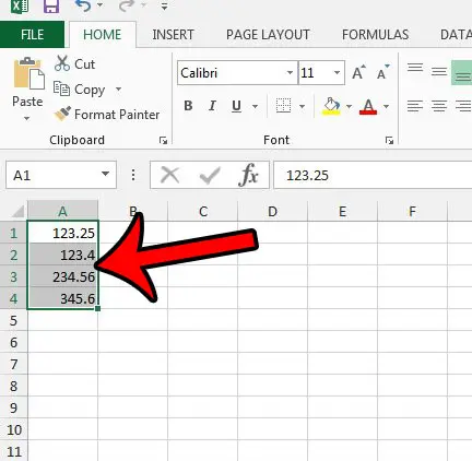
Step 2: Use your mouse to select the cells where you would like to use two decimal places.
You can select an entire row by clicking the row number at the left side of the sheet, an entire column by clicking the column letter at the top of the sheet, or you can select the entire sheet by clicking the button above row 1, and to the left of column A.

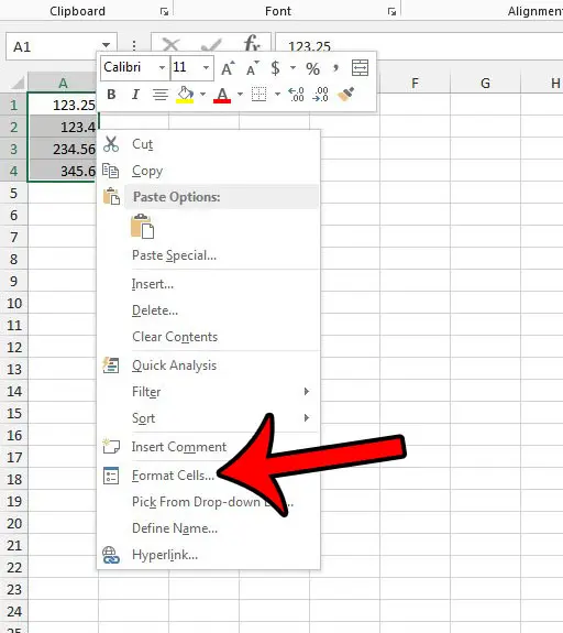
Step 3: Right-click one of the selected cells, then click the Format Cells option.

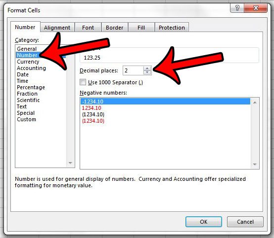
Step 4: Click the Number option in the column at the left side of the window, then confirm that the value in the Decimal places field at the center of the window is 2. You can then click the OK button at the bottom of the window to apply your changes.

Hopefully, this guide on how to show two decimal places in Excel has provided you with the instructions that you need in order to achieve your desired cell display.
Would you like the decimal separator to be a different symbol than the one currently being used? Click here and learn where you can change this setting.

Matthew Burleigh has been writing tech tutorials since 2008. His writing has appeared on dozens of different websites and been read over 50 million times.
After receiving his Bachelor’s and Master’s degrees in Computer Science he spent several years working in IT management for small businesses. However, he now works full time writing content online and creating websites.
His main writing topics include iPhones, Microsoft Office, Google Apps, Android, and Photoshop, but he has also written about many other tech topics as well.