Formatting data properly in Excel can solve a lot of problems that you might have with your formulas, or with readers understanding your data. But you may be wondering how to remove a dollar sign in Excel if you don’t want it included next to your data.
Properly applied cell formatting in Microsoft Excel can make it much easier for your audience to understand the data that you are presenting. For example, if the values in your cells are displaying monetary values, and you have them formatted as simple numbers, then the lack of commas, or inconsistent decimal places, can be problematic.
You can read our article about how to check cell format in Excel if you would like to know what format a cell is currently using.
But if you have already formatted your cells with the currency format, but find the dollar symbol that precedes the numbers to be unnecessary, then you might be wondering if that is something that you can adjust, while still keeping the rest of the currency formatting. Fortunately that is possible, and can be applied by following our short guide below.
How to Remove Dollar Sign in Excel
- Open your file.
- Select the cells to change.
- Right-click a selected cell and choose Format Cells.
- Click the Symbol dropdown and choose None.
- Click OK.
Our article continues below with additional information on removing the dollar sign in Excel, including pictures of these steps.
When you need to remove something from a cell that isn’t there because of formatting, then our tutorial on how to remove first character in Excel will show you a useful way to do so.
Adjust the Formatting for Currency Cells in Excel 2013 (Guide with Pictures)
The steps in this article will assume that the cells you want to modify are currently formatted as currency, and that you simply want to stop displaying the dollar symbol that is precedes the number. This article will show you how to keep the currency formatting, but remove the dollar sign from in front of the numerical value.
If you simply want to remove all of the formatting from your cells, this article will show you how.
Step 1: Open your spreadsheet in Excel 2013.
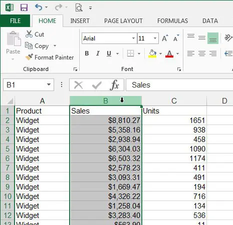
Step 2: Select the cells that you want to modify.
In the example below I am changing the formatting for an entire column, so I have simply clicked the column letter at the top of the spreadsheet to select the entire column.

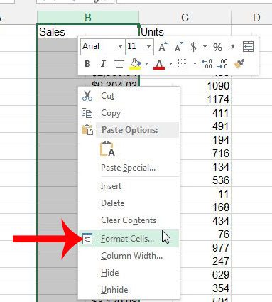
Step 3: Right-click on one of the selected cells, then click the Format Cells option.

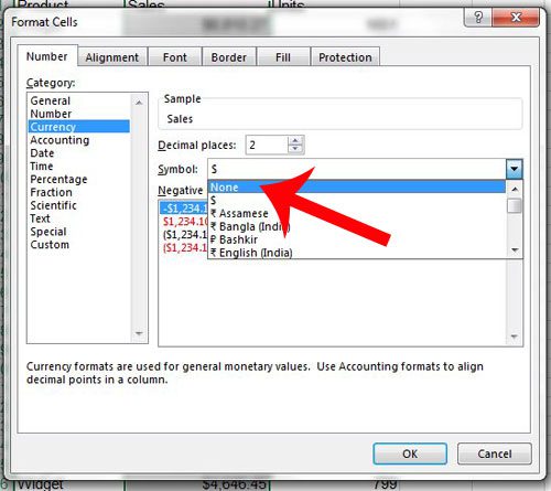
Step 4: Click the drop-down box to the right of Symbol, then click the None option.

Step 5: Click the OK button to apply your changes.
If the dollar signs were not added to your cells via Currency formatting, but were added manually, then the “Find and Replace” tool will likely be the best solution. Simply open Find and Replace, enter a “$” into the “Find” field, and leave the “Replace” field empty. You can then click “Replace All” and it will remove all of the dollar signs.
Are there hidden cells in your spreadsheet that you need to edit? Learn how to show hidden cells in Excel 2013 so that you can make changes to the data they contain.

Matthew Burleigh has been writing tech tutorials since 2008. His writing has appeared on dozens of different websites and been read over 50 million times.
After receiving his Bachelor’s and Master’s degrees in Computer Science he spent several years working in IT management for small businesses. However, he now works full time writing content online and creating websites.
His main writing topics include iPhones, Microsoft Office, Google Apps, Android, and Photoshop, but he has also written about many other tech topics as well.