Learning how to unhide a row in Excel 2013 can help to solve some confusing situations that arise when you know data is in a spreadsheet, but you cannot see it. People hide rows in Excel 2013 for a number of reasons, and data that might initially seem to be irrelevant, and was therefore hidden, could prove important a later time.
But when you are used to selecting a row if you need to make a change to it, such as if you want to increase the row height, you may encounter difficulty because the hidden row can not be selected. Fortunately it is possible to unhide a row in Excel 2013 by following the steps below.
One other thing that you might want to do with rows is make them taller. Our how to expand all rows in Excel guide can show you an easy way to do it to a lot of rows at once.
Unhiding Rows in Excel 2013
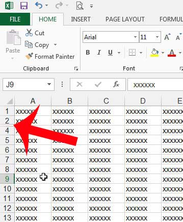
Our article below will teach you how to make hidden rows visible in Excel 2013. You will know that a row is hidden because a number (or numbers) will be skipped in the row labels at the left side of the spreadsheet. There will also be a small rectangle in place of where the row number should be, as in the image below.

Any cells in hidden rows that are referenced by formulas will still be valid. The cells in the hidden row are simply not visible on the spreadsheet until you follow our steps below to unhide the row. If you wish to learn how to hide rows in Excel 2013, you can read this article.
Step 1: Open the spreadsheet in Excel that contains the rows that you want to unhide.
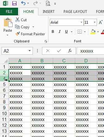
Step 2: Select the row numbers surrounding the row number(s) that you want to unhide. Note that you can also elect to select the entire spreadsheet by clicking the cell at the top-left corner of the spreadsheet. In the example image below row 3 is hidden, so I am selecting row 2 and row 4.

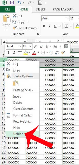
Step 3: Right-click one of the highlighted row numbers, then click the Unhide option.

You can visit Microsoft’s website here to learn more about unhiding rows.
Now that you know how to unhide a row in Excel 2013 you will be able to view or modify data that is included inside of the cells that had previously been hidden in a worksheet.
Printing a large spreadsheet in Excel 2013 can be a bit of a hassle, but you can make it easier to read by printing the top row on every page. This will make all of your pages much easier to read by repeating yoru column headers on each printed page.

Matthew Burleigh has been writing tech tutorials since 2008. His writing has appeared on dozens of different websites and been read over 50 million times.
After receiving his Bachelor’s and Master’s degrees in Computer Science he spent several years working in IT management for small businesses. However, he now works full time writing content online and creating websites.
His main writing topics include iPhones, Microsoft Office, Google Apps, Android, and Photoshop, but he has also written about many other tech topics as well.