Microsoft Excel gives you a lot of ways to store and edit the data in a worksheet.
In fact, there are so many different options that it can often be overwhelming when you are trying to figure out how to do something.
one useful option in Excel is the ability to hide some data ranges in your spreadsheet.
Our tutorial below will show you how to hide multiple rows in Excel if you don’t want that data ot be visible, but would still like ot keep it in the spreadsheet.
How to Hide More than One Row in an Excel 2013 Worksheet
- Open the worksheet in Excel 2013.
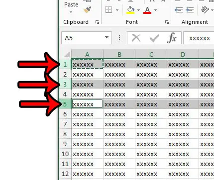
- Hold down the Ctrl key on your keyboard, then click each row number that you wish to hide.
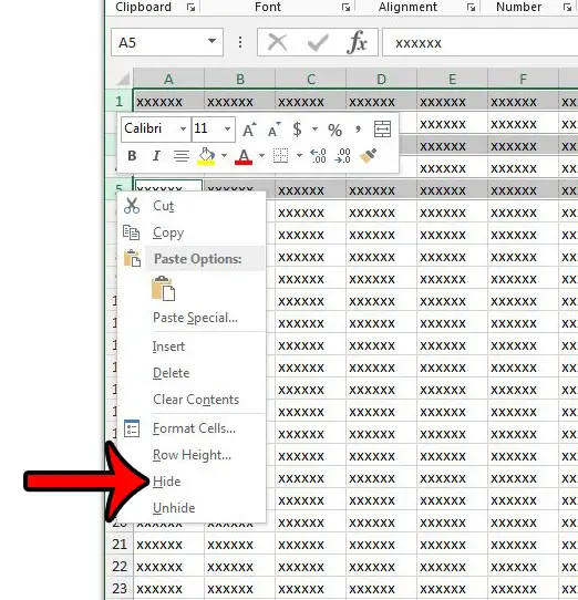
- Right-click one of the selected row numbers, then click the Hide option.
Our guide continues below with additional information about how to hide multiple rows in Excel, including pictures of these steps.
Check out our Excel freeze multiple rows guide if you want to keep some of your rows visible all the time, even as you scroll.
Informative spreadsheets often contain a large amount of data that you can use to answer related questions. But not every situation will require all of the data contained in that spreadsheet, so you may need to remove some unnecessary rows.
But deleting rows from your spreadsheet may not be appealing if you need that information later, so you may need a different alternative. Fortunately, you can hide rows in an Excel spreadsheet, even if you need to hide multiple separate rows.
If you would like to see your rows after hiding them in the steps below, then follow these steps to quickly unhide all of the hidden rows in your spreadsheet.
How to Use the Hide Option in Excel to Hide Multiple Rows (Guide with Pictures)
The steps in this article were performed in the Microsoft Excel 2013 version of the application, but will work in most other versions of Excel as well.
Step 1: Open your spreadsheet.
Step 2: Hold the Ctrl key on your keyboard, then click each row number that you wish to hide.
Row numbers are displayed at the left side of the spreadsheet, as identified in the image below.

Step 3: Right-click one of the selected row numbers, then click the Hide option.

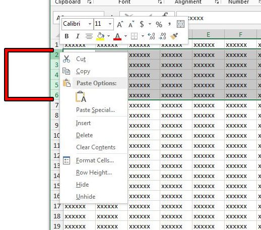
If you wish to hide a group of contiguous rows, then you can do so by clicking the top row number in the group, holding the Shift key, then clicking the bottom row in the group.
You can then right-click one of the selected row numbers and select the Hide option as well.

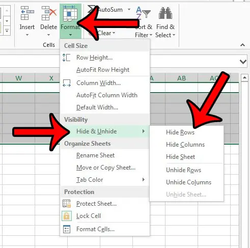
You can also hide a selection by clicking the Format button in the Cells section of the Home ribbon, click Hide & Unhide, then click the Hide Rows option.

Now that you know how to hide multiple rows in Excel you will be able to use this option when you have rows with data that you don’t want to edit, or if you are trying to clean things up visually and make it easier to manage certain parts of your data.
Do you know that you can also choose to print only a selection of rows from your spreadsheet as well? This can be a great way to reduce the amount of ink and paper that you use, while highlighting the most important information in your spreadsheet.

Matthew Burleigh has been writing tech tutorials since 2008. His writing has appeared on dozens of different websites and been read over 50 million times.
After receiving his Bachelor’s and Master’s degrees in Computer Science he spent several years working in IT management for small businesses. However, he now works full time writing content online and creating websites.
His main writing topics include iPhones, Microsoft Office, Google Apps, Android, and Photoshop, but he has also written about many other tech topics as well.