Do you find Excel 2013 to be kind of bland? While there are not a lot of default options for changing the theme of the program, there are some steps that you can take to make the program a little more cheerful while you are working in it. One of the ways that you can do this is by changing the gridline color.
Gridlines are the vertical and horizontal lines that separate the spreadsheet into cells. If you have never modified them, then they are probably gray. But you can follow our steps below and select a different color for the gridlines in your spreadsheet.
Using a Different Gridline Color in Excel 2013
Note that your gridlines will still not print by default. You will need to follow the steps in this article for your gridlines to print along with the data in your spreadsheet.
Step 1: Open Excel 2013.
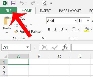
Step 2: Click the File tab at the top-left corner of the window.
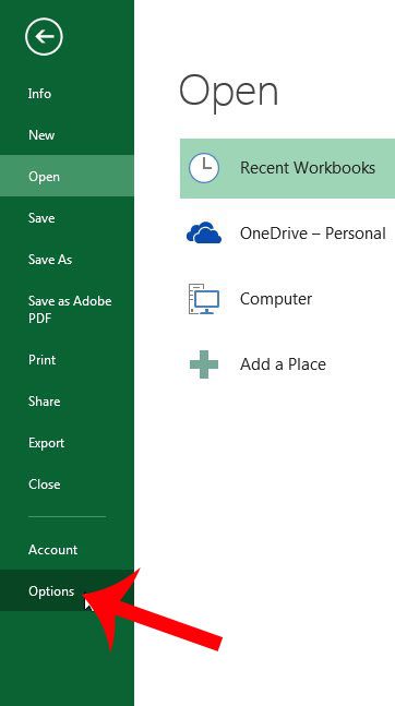
Step 3: Click the Options button in the column at the left side of the window.
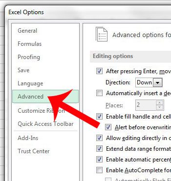
Step 4: Click Advanced in the left column of the Excel Options window that just opened.
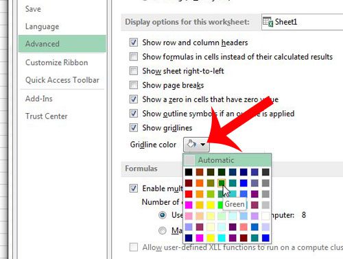
Step 5: Scroll down to the Display options for this worksheet section.
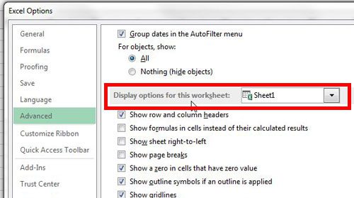
Step 6: Click the button to the right of Gridline color, then click the color that you want to use. You can then click the OK button at the bottom of the window to save your changes.
Now that you know how to change the gridline color in Excel 2013 you will be able to adjust the appearance of the worksheets that you edit on your computer and make them look a little less dull.
Do you have a row of headings that you want to print on every page of your Excel spreadsheet? Learn how with this article and make it easier for people to read your printed Excel files.

Matthew Burleigh has been writing tech tutorials since 2008. His writing has appeared on dozens of different websites and been read over 50 million times.
After receiving his Bachelor’s and Master’s degrees in Computer Science he spent several years working in IT management for small businesses. However, he now works full time writing content online and creating websites.
His main writing topics include iPhones, Microsoft Office, Google Apps, Android, and Photoshop, but he has also written about many other tech topics as well.