Microsoft Excel Create Table Guide

If you’ve ever used a worksheet in Excel that contained a table, then you’ve probably noticed how useful of a tool it can be. But if you’ve been trying to make one yourself but have been struggling to figure out how, then our Microsoft Excel Create Table guide below can point you in the right direction.

If you haven’t ever used the table tools in Microsoft Excel, then you might not even be aware of the fact that Excel can add tables to a spreadsheet.

Many people think of Excel spreadsheets in a manner similar to how they think of tables in a Microsoft Word or Microsoft Powerpoint document. Essentially it is thought of as a way to store data.

But as you become familiar with Microsoft Excel you start to realize all the formatting options available within the application, as well as all of the ways that you can sort and manipulate data.

Our tutorial below with show you how to add a table to a worksheet in Excel that includes the default table style, then we will discuss ways that you can change table styles and apply your own custom table style.

How to Make an Excel Table

1. Open your spreadsheet.
2. Select the data for the table.
3. Click the Home tab.
4. Click the Format as Table button.
5. Choose the table style.
6. Click OK.

Our guide continues below with additional information on creating Microsoft Excel tables, including pictures of these steps.

How to Add Excel Tables in a Microsoft Excel Spreadsheet (Guide with Pictures)

The steps in this article were performed in the desktop version of the Microsoft Excel for Office 365 version of the application.

Step 1: Open the Microsoft Excel workbook containing the data that you would like to turn into a table.

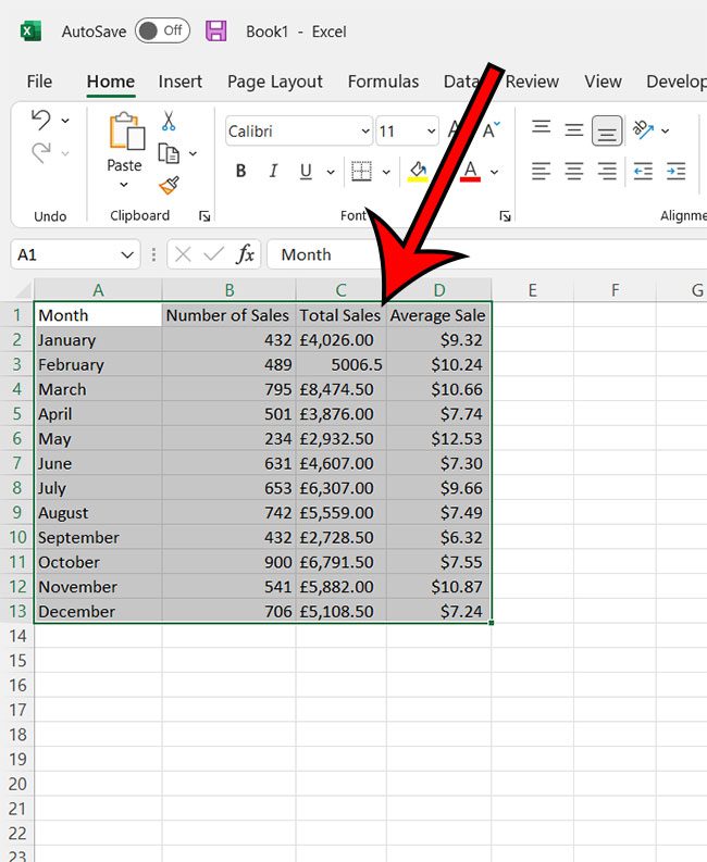
Step 2: Select the data to format as a table.

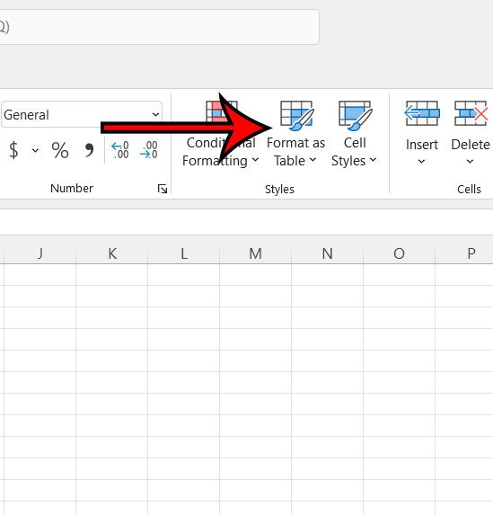
Step 3: Click the Home tab at the upper left corner of the window.

Step 4: Select the Format as Table button in the Styles group of the ribbon.

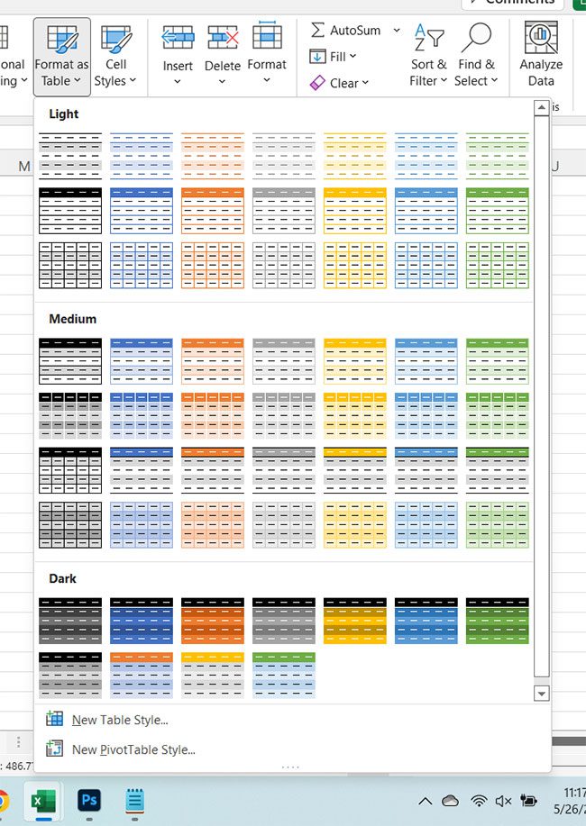
Step 5: Choose the desired table format for your existing table from the options in the table styles gallery.

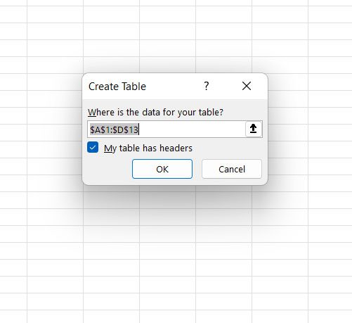
Step 6: Click the OK button on the Create Table dialog box to confirm that the data range is accurate.

You will also be able to check or uncheck the box next to My table has headers.

Now that you have your table data, it’s time to start working with the various table style options so that you can get the right type of new table style and table elements for your data range.

More Information on Working with an Excel Table and Adjusting Table Formatting in Excel

Once you have created your table you are going to see a new Table Design tab at the top of the window when you click inside the formatted table.

There is a lot of data and formatting choices that you can make here, especially in the Table Style Options group and the Table Styles group.

Inside the Table Style Options group you will find these options:

• Header Row
• Total Row
• Banded Rows
• First Column
• Last Column
• Banded Columns
• Filter Button

The various options that you will want to select here are going to depend on your data and how you are using the table.

For example, I almost always use the header row and banded rows, as well as the filter button. Since I am usually creating tables so that I can sort data where totals are important, I also like to use a total row that lets me get sums for the entire table columns.

There is only the Table Styles gallery inside of the table Styles group in the ribbon, but you can also click the down arrow with the horizontal line above it to expand that gallery, where you will see these options at the bottom of the dropdown menu:

• New Table Style – you can click this option and create your own custom style for the table if none of the default options are providing the look that you want.
• Clear – You can use this if you want to clear formats from the table, but leave the data in the table format. Note that this will not revert the table back to a regular range. it just gets rid of any styling applied to the table. You will still be able to filter and sort it like a regular Excel table.

After you have turned your data into a table, you might change your mind and decide that you want to remove table formatting. Luckily that is an option as well.

You simply need to click anywhere inside of the table, then click the Convert to Range button in the Tool group of the ribbon.

This should clear table formatting and remove all of the table features as it reverts your data back into standard Excel cells. Note that when you remove formatting, you will also lose any structured references that were made in formulas that referenced things inside of the table.

Conclusion

Hopefully, our Microsoft Excel create table guide has provided you with the information that you need to start formatting data as tables in your spreadsheets.

By customizing certain datasets as tables, you will have easier ways to sort and filter the important information to streamline your data processing needs.

It’s also helpful to familiarize yourself with the Excel removing table format process discussed above as well, in case you encounter a table that you need to turn back into a standard spreadsheet cell range.