To hide a column in Excel Online, click the column letter to select it, right-click it, and choose Hide. A double line between the neighboring column letters shows where the hidden column is. To bring it back, select the columns on both sides of that line, right-click, and choose Unhide.
Excel Online is now called Excel for the web. The browser steps come first, and a short section near the end covers the Windows desktop app. The steps follow Microsoft’s Hide or show rows or columns instructions. Hiding a column only removes it from view. To remove a whole sheet and its data instead, delete a worksheet tab in Excel Online.
You Need Edit Permission
- You need to be able to edit the workbook. If the file opened in a view-only mode, or the sheet is protected, the Hide option may be missing or grayed out.
- Hiding is not a privacy tool. The data stays in the workbook, and other people who can edit the file can show the column again.
- Other people may see the change. In a shared workbook, a column you hide may be hidden for the other people who open the file too, so let co-workers know if they rely on that column.
How to Hide Columns in Excel Online
- Open your workbook in Excel for the web. It opens in a browser tab from OneDrive or SharePoint.
- Click the letter at the top of the column you want to hide. The whole column is highlighted.
- To hide several columns that sit next to each other, drag across their letters. To add columns that are not side by side, hold Ctrl and click each letter.
- Right-click one of the selected column letters. On a touch screen, select and hold instead. A menu opens.
- Choose Hide.
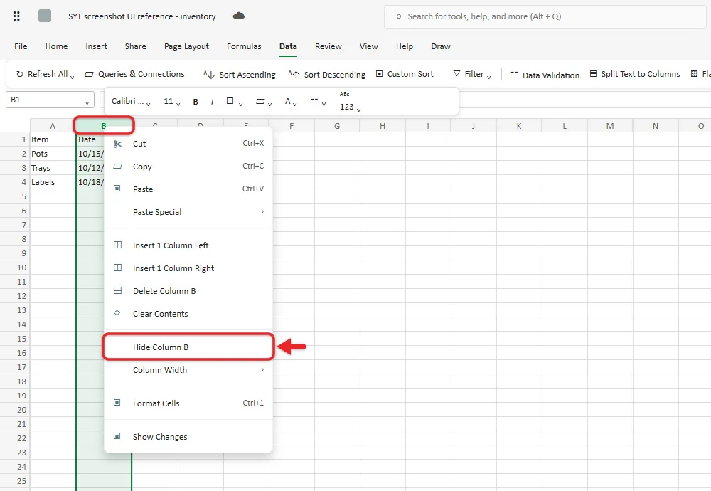
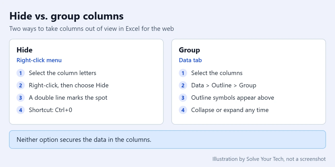
The selected columns disappear, and the column letters skip ahead. For example, if you hid column C, the headings read A, B, D, E. Microsoft notes that the double line between two columns is the sign that a column is hidden there.
Hide Columns With a Keyboard Shortcut
Microsoft’s keyboard shortcut list for Excel for the web includes shortcuts for hiding and showing columns and rows.
| Action | Shortcut in Excel for the web |
|---|---|
| Select the entire column | Ctrl + Spacebar |
| Hide columns | Ctrl + 0 |
| Unhide columns | Ctrl + Shift + 0 |
| Hide rows | Ctrl + 9 |
| Unhide rows | Ctrl + Shift + 9 |
Click any cell in the column and press Ctrl + 0 (zero) to hide that column. Because Excel for the web runs inside a browser, some key combinations can be claimed by the browser before Excel receives them. If a shortcut does nothing, or the browser reacts instead, Microsoft’s fix is to select Help > Keyboard Shortcuts in Excel for the web and turn on Override browser shortcuts. The right-click method above works either way.
How to Unhide Columns
- Find the double line between two column letters. That is where the hidden column sits.
- Select the columns on both sides of it. For example, drag across B and D to unhide C.
- Right-click the selection, or select and hold on a touch screen.
- Choose Unhide.
The hidden column reappears between its neighbors with its data intact. Microsoft gives a second way too: double-click the double line between the two columns. If you just hid the column by mistake, pressing Ctrl + Z to undo is usually the fastest fix.
Like hiding, width changes apply to the whole column, so here is what to do when you want to resize just one cell in Excel.
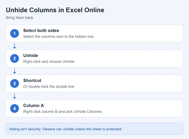
How to unhide column A
There is no column to the left of A, so you cannot select both sides. In Excel for the web, Microsoft’s Unhide the first column or row article says to right-click the column B header and pick Unhide Columns. For a hidden row 1, right-click the row 2 header and pick Unhide Rows. If you do not see those options, make sure you are right-clicking inside the header label itself and not in a cell.
Hide and Unhide Rows the Same Way
Rows work just like columns. Click the row numbers on the left side of the sheet, hold Ctrl to add rows that are not next to each other, then right-click and choose Hide. A double line between two row numbers marks the hidden rows. To show them, select the rows above and below, right-click, and choose Unhide, or double-click the double line.
If you only want a header row or first column to stay on screen while you scroll, hiding is the wrong tool. Use Freeze Panes in Excel for that.
Group Columns So You Can Collapse Them
If you hide and show the same columns often, grouping may suit you better. A group, which Excel also calls an outline, adds a small symbol above the columns that collapses or expands them with one click. You can group rows and columns in Excel for the web.
- Select the columns you want to collapse.
- Go to Data > Outline > Group > Group, then select Columns if Excel asks.
- Use the outline symbol above the group to hide the columns, and again to show them. Microsoft also lists Alt + Shift + – to hide a group’s detail and Alt + Shift + = to show it.
To remove a group, select the columns and go to Data > Outline > Ungroup > Ungroup. The exact layout of the Data tab can vary with your ribbon view and window width, so look for the Outline or Group button if the path looks slightly different.
Keep Hidden Columns Hidden When Sharing
Anyone who can edit the workbook can unhide a column in a few clicks. To make that harder, hide the columns first and then protect the sheet. In Microsoft’s Protect a worksheet article, the option named Format columns is the one that controls column formatting commands, including changing column width and hiding columns.
Before you protect a sheet: by default the entire sheet is locked once protection is on, so other people cannot edit any cell unless you unlock ranges for them. If you set a password, keep a record of it, because you need it to turn protection off.
- Hide the columns using the steps above.
- Select Review > Manage Protection. A task pane opens on the side.
- Turn on Protect sheet.
- If people need to type in certain cells, select Unlocked ranges and add those ranges. In the Options section, leave the column formatting option turned off so others cannot hide or unhide columns.
- Optionally set a sheet password so that others cannot switch protection off.
To undo this, go back to Review > Manage Protection and turn off Protect sheet. Microsoft also offers Review > Pause Protection, which lifts protection for your own editing session while it stays on for everyone else.
Microsoft is clear that worksheet protection is not intended as a security feature. It discourages changes, but it does not encrypt anything. For data that certain people must never see, keep it in a separate workbook that you do not share with them. If the goal is only to stop edits, you can also make an Excel spreadsheet read-only for others.
Unhide Columns in Desktop Excel
In desktop Excel on Windows, select the column letters on both sides of a hidden block. For example, if B through D are hidden, drag across A through E. Right-click a selected header and choose Unhide, then check that the missing letters and data appear. For several separate hidden blocks, select ranges enclosing each gap; hold Ctrl while adding separate ranges. Microsoft’s hide/unhide guide documents selecting the neighboring columns and using Unhide.
To show every hidden column, click the sheet’s Select All button where the row numbers and column letters meet, then choose Home > Format > Hide & Unhide > Unhide Columns. Check the column letters, including column A. This only changes what’s visible, not the cell values. A protected worksheet may block column formatting; if Unhide does nothing, check whether the sheet is protected. Save a copy before changing the layout of a complex workbook.
To show only column A in desktop Excel, type A1 in the Name Box beside the formula bar, press Enter, then choose Home > Format > Hide & Unhide > Unhide Columns. Microsoft’s first-column guide documents this method.
If Hide or Unhide Isn’t in the Menu
- Hide or Unhide is not in the menu. Right-click the column letter at the top of the sheet. Microsoft’s instructions use the selected column headers, and its tip for column A says the option appears when you right-click inside the header label.
- Hide and Unhide are grayed out. The sheet is probably protected. Go to Review > Manage Protection and turn off Protect sheet, or use Pause Protection. You need the password if one was set. If someone else owns the file, ask them.
- You cannot change anything at all. The workbook may have been shared with you as view-only. Ask the owner for edit access, or save your own copy and work in that.
- Unhide did nothing. Make sure the selection includes a column on each side of the double line. Selecting only one neighbor is not enough, except for column A, where you right-click column B.
- The column is still missing and there is no double line. The columns may be grouped and collapsed instead of hidden. Look for an outline symbol above the column letters and select it to expand the group.
- Ctrl + 0 does not hide the column. Turn on Override browser shortcuts under Help > Keyboard Shortcuts, or use the right-click menu.

Excel Online Column Questions
Does hiding a column delete the data in it?
No. Hiding only takes the column out of view. The cells and their contents stay in the workbook, and they come back unchanged when you choose Unhide.
Will hidden columns print?
Hidden columns are generally left out of a printout. Hiding rows and columns is a way to show only the data you need to see or print. Check the print preview before you print to confirm the page looks the way you expect.
Can I hide several columns at once in Excel Online?
Yes. Drag across the column letters to select a block, or hold Ctrl and click separate column letters, then right-click one of them and choose Hide. All selected columns are hidden together.
How do I unhide all columns at once?
Select a range of columns that spans every hidden one, for example by dragging from the first visible column letter to the last, then right-click the selection and choose Unhide. Every hidden column inside the selection is shown. If column A is hidden too, right-click the column B header and choose Unhide Columns.
Can other people see a column I hid in a shared workbook?
They will not see it on screen, but anyone with edit access can unhide it. Protecting the sheet after hiding makes that harder, though sheet protection is not a security feature. Keep truly private data in a separate file.
Do these steps work in the Excel desktop app?
Yes. The right-click Hide and Unhide steps are the same in Excel for Windows and Mac. The desktop app also has the commands on the ribbon under Home > Format > Hide & Unhide.
More Excel Guides
Now that the extra columns are out of the way, these guides cover other common Excel tasks. If you also use Google’s spreadsheet app, here is how to hide a column in Google Sheets.
- How to sort by date in Excel Online
- How to AutoFit columns and rows in Excel
- How to download a copy of an Excel Online file

Matthew Burleigh is the founder, head writer, and editor of Solve Your Tech, which he launched in 2012. He has written technology tutorials since 2008 and worked in IT since 2003, including small-business support, IT management, and consulting. He holds Bachelor’s and Master’s degrees in Computer Science from Arizona State University.
Matthew writes practical guides for Windows, iPhone and iPad, Microsoft Office, Outlook, Google apps, and Android. Solve Your Tech’s guides are checked step by step against the device or app maker’s own documentation and tested on his own devices whenever he has the hardware or software, with clear steps, sources, and update dates.
Read more about Matthew and how Solve Your Tech writes and updates its guides, or report a correction.