Entering all of the data into your spreadsheet and using it to create a pivot table in Excel is a great way to manage your data.
But you might need to update some of that information, which can leave you looking for a method for how to refresh a pivot table in Excel.
Fortunately, this is something that many pivot table users need to do, so Excel has a quick way for you to perform this data refresh.
How to Refresh Microsoft Excel 2013 Pivot Table Data
- Open your spreadsheet.
- Edit your data as needed.
- Select the pivot table tab.
- Click inside the table.
- Choose the Analyze tab.
- Click Refresh.
Our guide continues below with additional information on how to refresh a pivot table in excel, including pictures of these steps.
Pivot tables in Excel 2013 are very helpful tools that let you quickly view the data from your spreadsheets in whatever way you need. Pivot tables can be easily manipulated and sorted without requiring you to edit or delete any of the important original data that is in your spreadsheet.
But you might discover that the information you are seeing in your pivot table needs to be updated, either because it has been changed, or you noticed that it was incorrect.
However, that data may not be updating automatically in your pivot table once you change it in the source spreadsheet.
Luckily there is a way to refresh your pivot table after you have updated the spreadsheet data on which the pivot table was based.
Our tutorial on creating tables in Excel can show you some other ways to create and use tables in your spreadsheets.
How to Update an Excel 2013 Pivot Table (Guide with Pictures)
The steps in this article were performed in Microsoft Excel 2013. This guide assumes that you have already created a pivot table, but that you have recently updated the data that was used to generate the pivot table. Following these steps will cause the pivot table to check the source data again and update itself accordingly.
Step 1: Open your spreadsheet in Excel 2013.
Step 2: Make any changes to your original source data that you would like to be reflected in your pivot table.
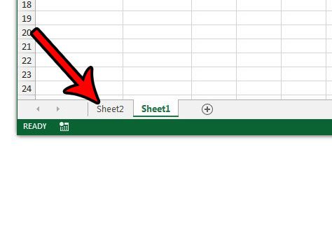
Step 3: Select the tab at the bottom of the worksheet that contains the pivot table.

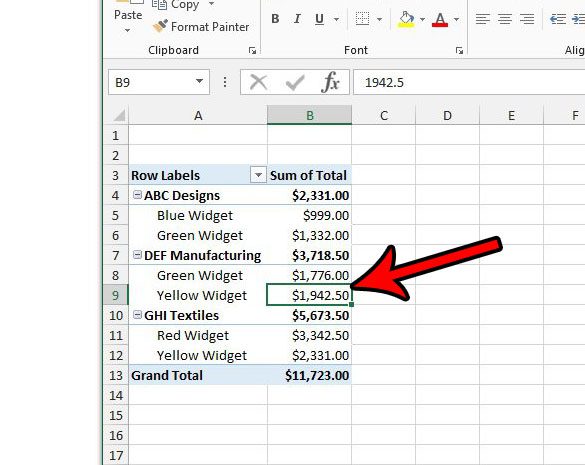
Step 4: Click inside the pivot table.

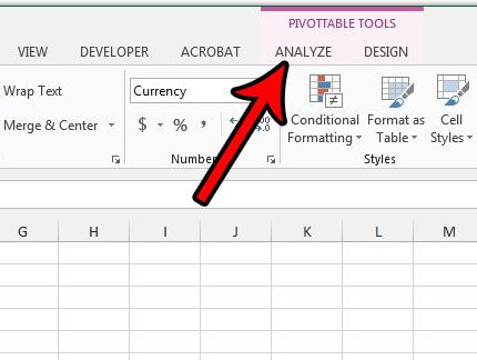
Step 5: Click the Analyze tab at the top of the window.

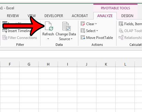
Step 6: Click the Refresh button.
Note that, rather than clicking the Refresh button in the ribbon to update your pivot table data, you can choose to press the F5 key on your keyboard instead.

Now that you know how to refresh a pivot table in Excel you will be able to create one in your workbook and add more information to the sheet where the table is generating its data.
Do you need to print your spreadsheets, but something is preventing that from being simple? Learn how to optimize spreadsheets for printing in Excel and save yourself some frustration.
Additional Sources

Matthew Burleigh has been writing tech tutorials since 2008. His writing has appeared on dozens of different websites and been read over 50 million times.
After receiving his Bachelor’s and Master’s degrees in Computer Science he spent several years working in IT management for small businesses. However, he now works full time writing content online and creating websites.
His main writing topics include iPhones, Microsoft Office, Google Apps, Android, and Photoshop, but he has also written about many other tech topics as well.