While there is a lot that you can do to sort and total data in normal cells of an Excel spreadsheet, the Pivot Table tool can give you a lot more options and flexibility.
But if you’ve never used them before, you may be wondering how to create a pivot table in Excel 2010.
How to Make an Excel Pivot Table
- Open the spreadsheet.
- Select the data.
- Click Insert.
- Choose PivotTable, then PivotTable again.
- Click OK.
- Check the fields to include.
Our guide continues below with additional information on how to create a pivot table in excel 2010, including pictures of these steps.
I was recently downloading a lot of CSV orders from a customer, which I then combined into one file using the CSV file combination process in this article.
However, all of the data from those orders was itemized, and our production team needed each item combined into one line so that they knew how much of each item to produce.
Manually going through thousands of lines of data, even when it is sorted, is a hassle. Pivot tables provide the perfect solution to this problem.
Read our guide on creating tables in Excel for more ways that you can use Microsoft’s table tools to sort and filter data.
How to Generate a Pivot Table in Microsoft Excel (Guide with Pictures)
the steps in this article were performed in the Microsoft Excel 2010 version of the application but will also work in other versions of Excel too.
Step 1: Open your Excel file in Excel 2010.
Step 2: Highlight all of the data that you want to include in the pivot table.
Don’t highlight any column headings, as that will complicate the process.
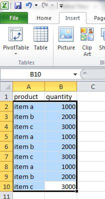
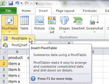
Step 3: Click “Insert” at the top of the window, click “Pivot Table,” then click “Pivot Table” again.
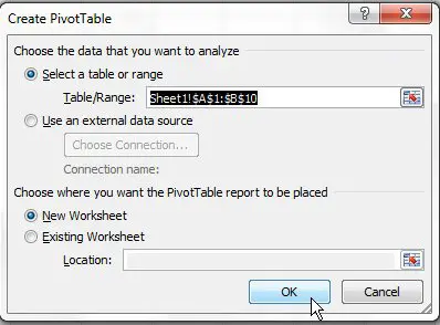
Step 4: Click the “OK” button in the pop-up window to create the pivot table on a new sheet.
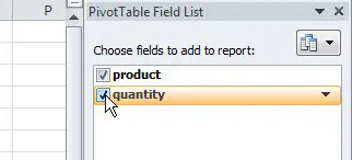
Step 5: Check the box to the left of each column at the right side of the window.
Each value will be combined into one line, showing the total associated quantity for that value.
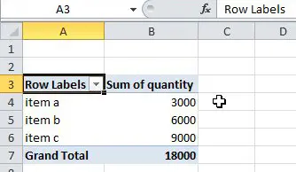
Now that you know how to create a pivot table in Excel 2010, you can start to use it more and more often and become comfortable with applying it to almost any situation where it can make large amounts of data easy to manage.
While a pivot table can help simplify the presentation of certain types of data, you may need to combine some of the data in its columns. Find out how to use the concatenate formula in Excel and quickly combine multiple columns into one.

Matthew Burleigh has been writing tech tutorials since 2008. His writing has appeared on dozens of different websites and been read over 50 million times.
After receiving his Bachelor’s and Master’s degrees in Computer Science he spent several years working in IT management for small businesses. However, he now works full time writing content online and creating websites.
His main writing topics include iPhones, Microsoft Office, Google Apps, Android, and Photoshop, but he has also written about many other tech topics as well.