How to Make Excel Continue to Count Up for Each Row

You typed 1 in a cell, dragged it down the column, and got a long line of 1s instead of 1, 2, 3. Type 1 and 2 in the first two cells, select both, and drag the fill handle down. Excel now has a pattern to follow, so it counts up.

These steps are for Excel for Microsoft 365, 2024, 2021, 2019 and 2016 on Windows. Which method suits you depends on what happens to your rows later.

Which Numbering Method to Use

Excel has no numbering button. Microsoft’s page on numbering rows offers typed series and formulas, and each behaves differently once the sheet changes. The biggest difference is between fixed numbers, which sit in the cell like anything you type, and formulas, which recalculate.

Method	After sorting	After deleting a row	New rows
Fill handle or Fill Series	Fixed numbers move with their rows	A gap stays until you refill	Not numbered
=ROW(A1)	Renumbers top to bottom	Microsoft warns the sequence can be interrupted	Fill the formula in
=ROW()-1	Should renumber; check on a copy	Should stay continuous; check on a copy	Fill the formula in
=SEQUENCE()	Not documented; check on a copy	Not documented; check on a copy	Change the row count
Excel table with a number column	Should renumber with a ROW formula; check on a copy	Should stay continuous; check on a copy	Rows added at the end are numbered
=A2+1	Can scramble the sequence	Can show #REF!	Fill the formula in

A quick rule: use the fill handle for a one-time list you won’t rearrange, and a table if the list keeps growing. If each number has to stay attached to one record, such as an invoice line, use fixed numbers, because formula numbers always count from the top.

Count Up With the Fill Handle

The fill handle is the small square at the bottom-right corner of a selected cell. One number gives Excel nothing to detect, so it copies the number. Two numbers show the step between them.

1. Click the first cell of the column and type your starting number, such as 1.
2. Type the next number, such as 2, in the cell below it.
3. Select both cells.
4. Point at the fill handle until the pointer changes, then drag down to the last row you need. Excel previews the values as you drag.

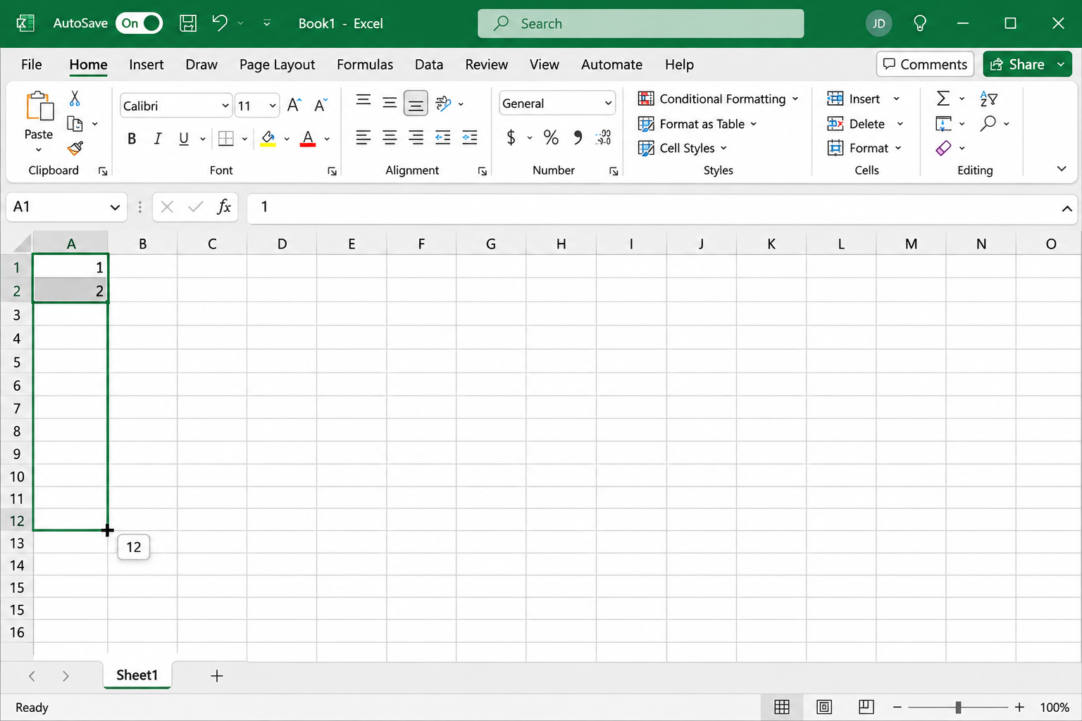
The two numbers set the step, so 2 and 4 counts by twos, and 5 and 10 counts by fives. Dragging up or left makes the sequence decrease. To choose a pattern from a menu when you let go, drag with the right mouse button instead.

Two shortcuts are widely used, though the Microsoft pages on this topic don’t describe either one, so try them on a spare sheet. Holding Ctrl while dragging a single cell is commonly used to make it count instead of copy. Double-clicking the fill handle fills down as far as the data in the next column runs, and it only works when that adjacent column has data.

If the Fill Handle Is Missing

1. Select File, then Options.
2. Select the Advanced category.
3. Under Editing options, turn on Enable fill handle and cell drag-and-drop.

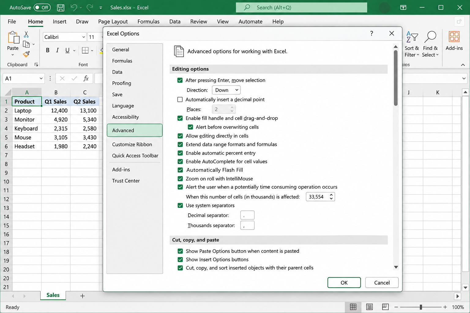
4. Leave Alert before overwriting cells on, so Excel warns you before a drag replaces existing data.

Fill a Set Count With the Series Command

Dragging down 5,000 rows is miserable. The Fill command’s Series dialog lets you type the step and the stopping point, and you drag nothing.

1. Type the starting number in the first cell and keep that cell selected.
2. On the Home tab, in the Editing group, select Fill, then Series.
3. Under Series in, choose Columns, and leave Type set to Linear.
4. Enter a step value of 1 and a stop value equal to your last number, such as 500.

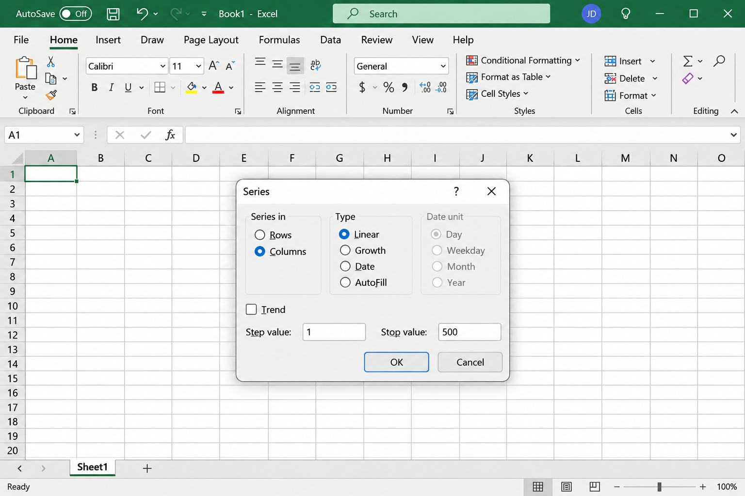
5. Select OK.

Excel stops at the stop value, however long the sheet is. For decimals, use a step value of 0.5. Like the fill handle, this writes fixed numbers that won’t update later.

Number Rows With the ROW Function

The ROW function returns a row number, which makes it a quick way to get numbers that recalculate. Give it a cell reference and it reports that cell’s row. Leave the parentheses empty and it reports the row holding the formula.

1. In the first cell of your number column, type =ROW(A1) and press Enter. It returns 1, whichever row it sits in.
2. Drag the fill handle to the end of the range. The reference moves down a row each time, so you get 2, 3, 4 and so on.

If your list has headers, the other form often reads more clearly. In a sheet with one header row and data starting in row 2, =ROW()-1 returns 1 in row 2. With three header rows and data starting in row 4, use =ROW()-3. Plain =ROW() returns the sheet row, so on its own it would start at 2 here, not 1.

Microsoft confirms that =ROW(A1) numbers update when you sort, and warns that adding, moving or deleting rows can interrupt the sequence. One reason is that each of these formulas points at a specific row, and deleting a row a formula refers to returns #REF!. Because =ROW() doesn’t point at another cell, deleting a row should simply close the gap, but no Microsoft page spells that case out, so test it on a copy before you rely on it. A newly inserted row starts empty either way: after you add a row in Excel, fill the formula into it from the row above.

For codes instead of plain numbers, =TEXT(ROW(A1),"000-000") starts a list at 000-001. Drag it down the same way.

Use SEQUENCE in Current Excel

With the SEQUENCE function, one formula produces the whole list. It works in Microsoft 365, Excel 2024 and Excel 2021 on Windows and Mac, and in Excel for iPad, iPhone and Android. Excel 2019 and 2016 don’t have it.

The format is =SEQUENCE(rows,[columns],[start],[step]), and the optional parts default to 1. Type the formula in the top cell only and the results spill into the cells below:

• =SEQUENCE(500) counts from 1 to 500.
• =SEQUENCE(10,1,100,5) gives ten rows starting at 100 and going up by 5.

To size the list from your data, try =SEQUENCE(COUNTA(B2:B100)), which makes one number for each filled cell in that range. This is a formula built for this situation and not a Microsoft example, and blank cells inside the range will throw the count off, so check it on a copy.

Two limits to plan for: only the top cell of the results can be edited, and the cells below it must be empty. Spilled formulas also aren’t supported inside Excel tables, so keep SEQUENCE in the plain grid outside one.

Keep Numbering New Rows With an Excel Table

For a list that keeps growing, a table does the most work. Microsoft states that rows added at the end of a table are numbered in sequence once you’ve converted the range.

1. Click any cell in your list.
2. On the Home tab, select Format as Table and pick a style. Pressing Ctrl+T, which opens the Create Table dialog, also works.
3. Check that My table has headers is selected if your first row holds headings, then select OK.
4. In the first data cell of your number column, type =ROW()-ROW(Table1[#Headers]), using your own table’s name in place of Table1, and press Enter.

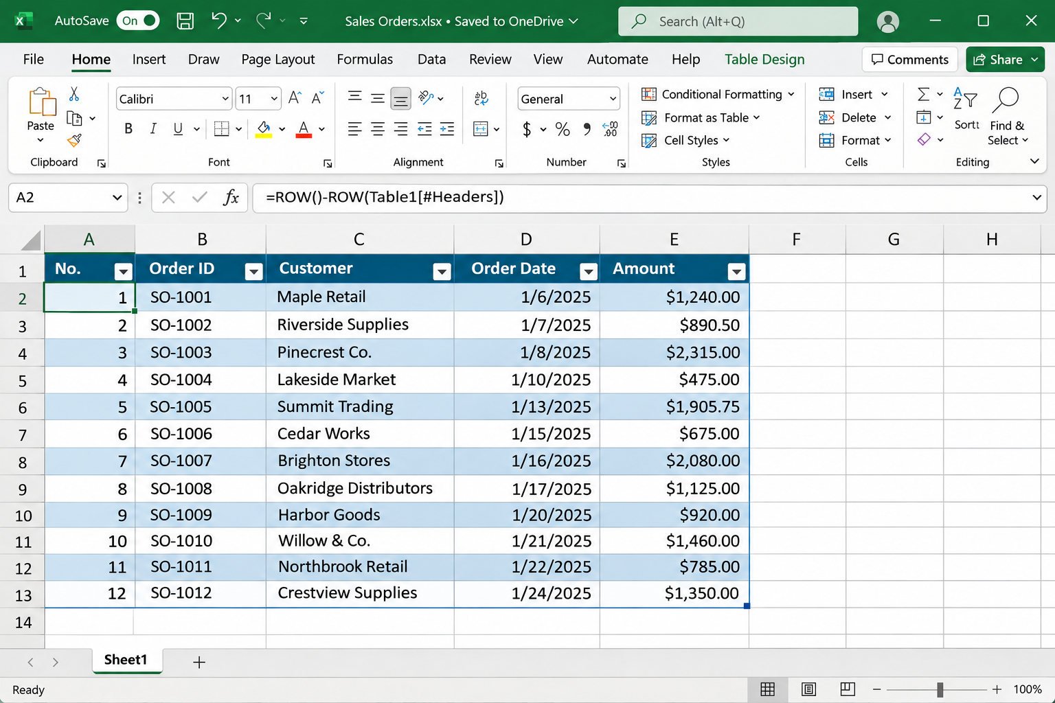
Excel expands a formula entered in a table column down the rest of that column for you. The structured formula comes from common practice and isn’t on Microsoft’s pages, so if it gives you trouble, =ROW()-1 does the same job for a table whose header sits in row 1.

Number Only Filled or Visible Rows

Plain row numbers count everything. These formulas count selectively, and all three assume item names in column B, starting in row 2. The blank-row and per-item versions are common spreadsheet practice and not Microsoft examples, so try them on a copy.

• Skip blank rows: =IF(B2<>"",COUNTA($B$2:B2),"") numbers a row only if column B has something in it. Blank rows stay blank and the count picks up afterward.
• Count only visible rows: =SUBTOTAL(3,$B$2:B2) renumbers 1, 2, 3 down whatever a filter shows, because SUBTOTAL always skips filtered-out rows. If you also hide rows by hand, use =SUBTOTAL(103,$B$2:B2). =AGGREGATE(3,5,$B$2:B2) is similar: in AGGREGATE, 3 is the count and 5 ignores hidden rows.
• Count each item separately: =COUNTIF($B$2:B2,B2) returns a running count per value. If Widget appears three times in a shipping list, its rows show 1, 2 and 3.

The dollar signs lock the top of the range while the bottom moves down with each row, and that growing range is what makes the count rise.

Count With the Previous Cell

You can also add to the cell above. With a starting number in A2, type =A2+1 in A3 and fill it down. Change the amount for other steps, such as =A2+5 or =A2+0.5.

This is the most fragile option. Each cell depends on the one above, so sorting can scramble the sequence (Microsoft notes that formula results in sorted data might change when the sheet recalculates), and deleting a row can leave #REF! errors below it. Save it for sheets you won’t rearrange.

Lock the Numbers and Handle Excel for Mac

To stop formula numbers from changing, turn them into plain values: select the column, copy it, then press Ctrl+Alt+V to open Paste Special and choose Values in the same spot. This is the right move before you sort a list whose numbers must stay with their records.

On a Mac, the two-value method works the same way. Microsoft’s series page for Excel 2024 and 2021 for Mac also describes the Auto Fill Options button that appears after filling, with Copy Cells, Fill Formatting Only and Fill Without Formatting choices. Menu locations can differ from Windows.

When Numbering Goes Wrong

• Every cell shows the same number: you dragged one cell. Add a second value and select both before you drag, or select the Auto Fill Options button that appears after the fill and choose Fill Series if it’s listed.
• You can’t grab the handle: turn it back on in File, Options, Advanced, as described earlier.
• Numbers are out of order after edits: select two correctly numbered cells at the top and drag the fill handle to the end of the range, which is Microsoft’s own fix.
• The list starts at the wrong number: you’re probably using =ROW() without subtracting the header rows.
• #NAME? appears with SEQUENCE: your Excel version may not include the function, so use ROW or the fill handle.
• #SPILL! appears with SEQUENCE: something is in the cells below, or the formula is inside a table. Select the cell, choose Select Obstructing Cells from the error alert and clear those cells, or move the formula out of the table.

More Row Numbering Questions

Once the numbers are in, a useful next move is to freeze the panes so that the column stays in view as you scroll, or total a column beside it. If you’re working with text patterns and not numbers, Flash Fill is the tool to look at.