Your boss wants one line per region from a 2,000-row sales sheet, not the whole list pasted into an email. To copy only the subtotals in Excel, sort by the column you group on, add totals with Data > Subtotal, click outline level 2, select the data, choose Home > Find & Select > Go To Special > Visible cells only, then copy and paste. These steps cover desktop Excel for Windows in Microsoft 365 and recent versions.
Why a Normal Copy Brings Back Every Row
When you collapse an outline to show only totals, the detail rows are hidden, not gone. If you select the block and press Ctrl+C, Excel copies the hidden rows along with the visible ones, so the paste fills 2,000 rows instead of a handful. The Visible cells only option in Go To Special fixes this by turning your selection into just the rows you can see. That one extra step is the whole trick, and it has to come after you collapse the outline, not before.
Step 1: Sort the Data and Add Subtotals
The Subtotal command inserts a total each time the value in your grouping column changes. If the data isn’t sorted, the same region shows up in several scattered groups and you get several totals for it.
- Make sure the list has one header row and no blank rows or columns inside it.
- Click any cell in the grouping column (for example, Region) and select Data > Sort A to Z.
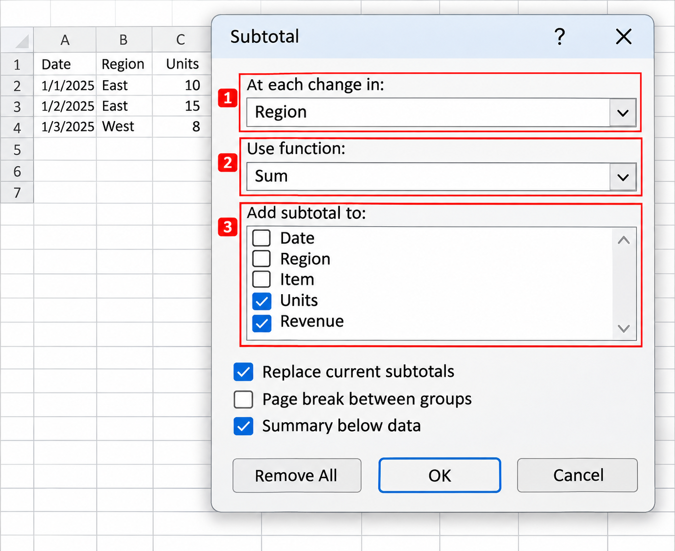
- Click any cell in the list and select Data > Subtotal (in the Outline group).
- In At each change in, pick the column you sorted on.
- In Use function, pick Sum (or Count, Average, Max and so on).
- Under Add subtotal to, check every column you want totaled, such as Units and Revenue.
- Leave Summary below data checked so each total sits under its group, and select OK.
Excel adds a row such as “North Total” after each group and a Grand Total at the bottom. Outline buttons labeled 1, 2 and 3 appear to the left of the row numbers.
Need totals by region and then by sales rep inside each region? Sort by Region, then Rep. Add the Region subtotals first, then open Subtotal again, choose Rep and uncheck Replace current subtotals so the first set stays. The outline then has four levels instead of three.
Step 2: Collapse the Outline to the Totals
Click the 2 button at the top left of the outline area. Excel hides the detail rows and shows only the subtotal rows plus the Grand Total. Level 1 shows the Grand Total alone, and the highest number shows everything. With nested subtotals, level 2 shows the region totals and level 3 adds the rep totals, so pick the level that matches the summary you want.
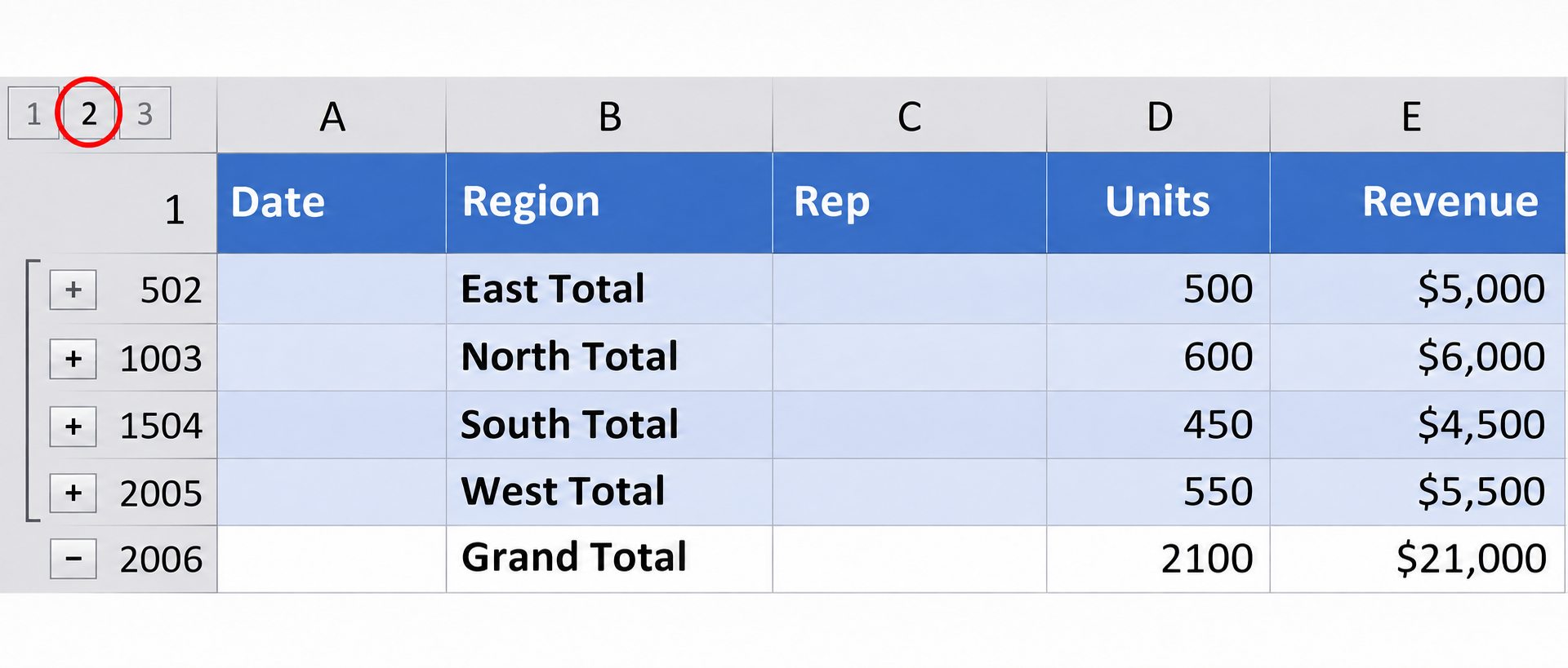
The Grand Total row is part of the level 2 view. If you don’t want it in the copy, leave its row out when you select in the next step. Note that Excel calculates the Grand Total from the detail data, not by adding up the subtotal rows.
Step 3: Select Only the Visible Cells
- Select the collapsed block, from the header row down to the Grand Total, across the columns you want to copy.
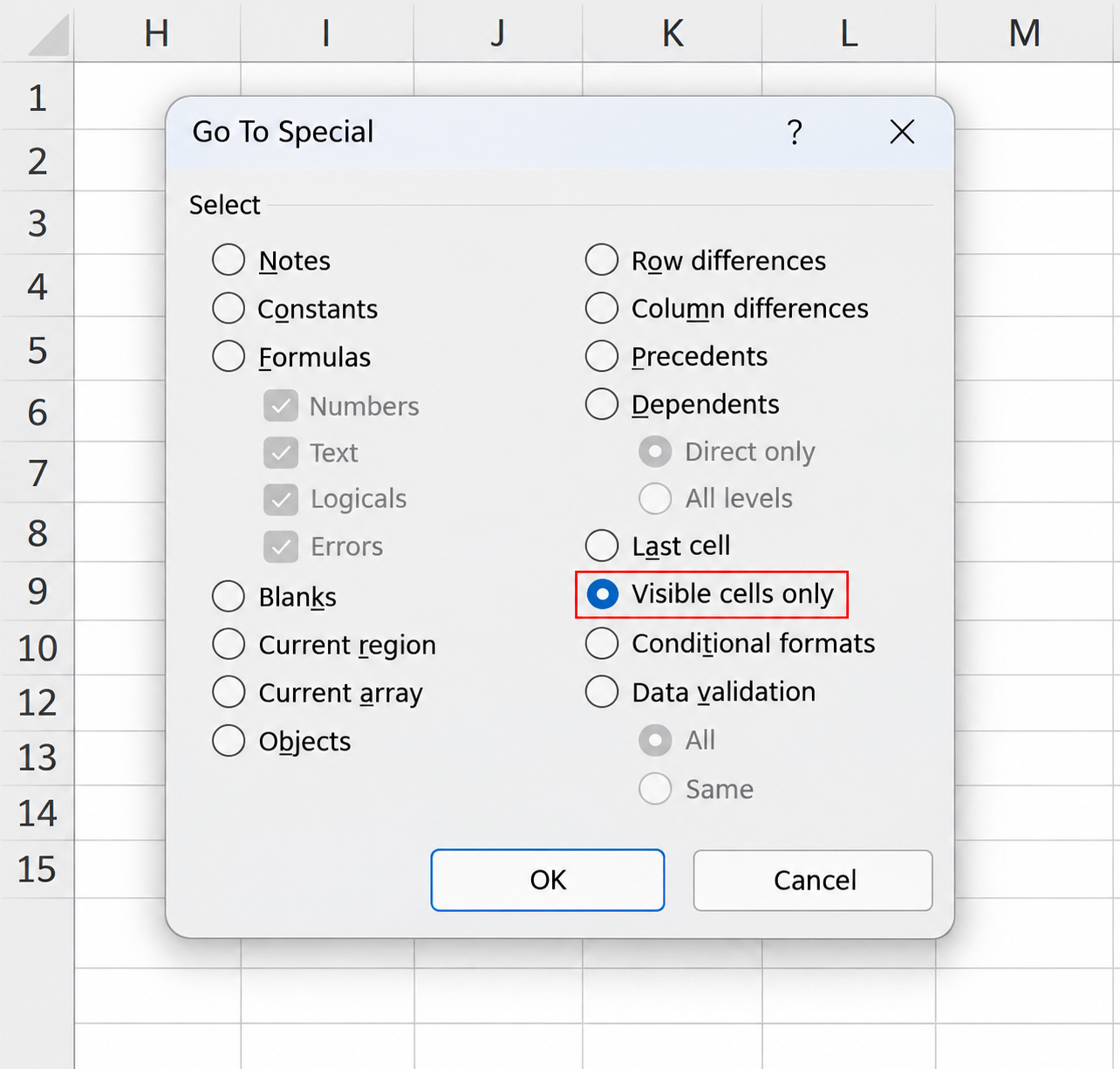
- Select Home > Find & Select > Go To Special. You can also press F5 and select Special.
- Choose Visible cells only and select OK.
The selection now shows thin white lines between the subtotal rows, a sign that Excel has broken it into separate pieces. Many people use Alt+; (Alt and the semicolon key) as a shortcut for Visible cells only; Microsoft’s main shortcut list doesn’t include it, so if it doesn’t work in your version, use the menu route above.
Step 4: Copy, Then Paste the Totals as Values
- Press Ctrl+C. A moving border appears around the visible rows.
- Go to a new sheet (or a blank area) and click the cell where the top-left corner should land.
- Press Ctrl+Alt+V to open Paste Special, choose Values and select OK. A plain Ctrl+V also works if you just want to see the rows.
Why values? Each total is a SUBTOTAL formula that points at the detail rows above it. Pasted as formulas into a new sheet, the relative references shift with the paste position, so they point at the wrong cells or past the top of the sheet, which shows up as #REF! errors, zeros or wrong numbers. Pasting values gives you fixed numbers you can email, chart or drop into a report. Formatting such as bold totals doesn’t come along with Values; use Paste Special again with Formats if you want it.
Worked example: Elena’s sheet has 2,000 orders across four regions with columns for Date, Region, Rep, Units and Revenue. After sorting by Region and adding Sum subtotals to Units and Revenue, level 2 shows five rows: East Total, North Total, South Total, West Total and Grand Total. She selects A1:E2006, applies Visible cells only, copies, and pastes values into a sheet named Summary. The result is six rows (header plus five totals), ready to paste into her email.
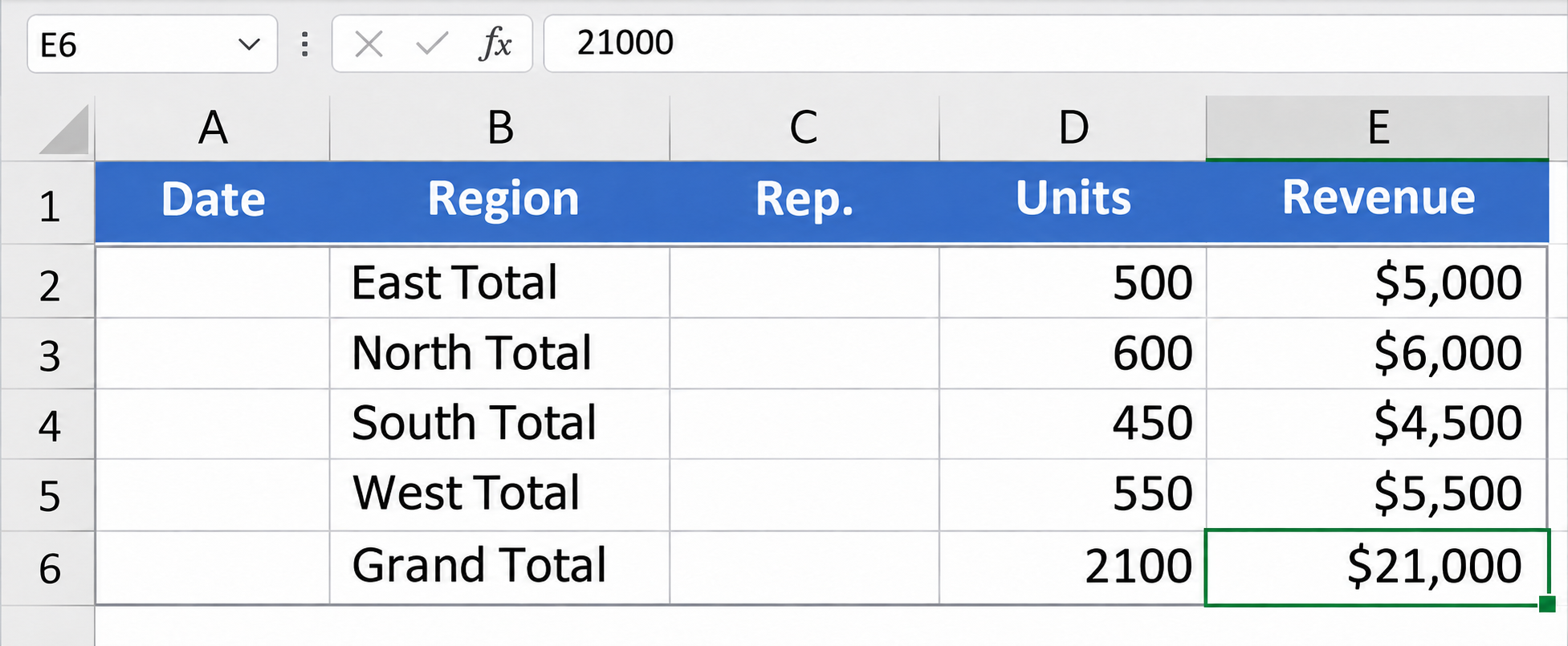
Tip: the Date and Rep columns are empty on total rows, so you can delete those columns in the summary, or select only the Region, Units and Revenue columns in step 3 if they sit next to each other.
If Your Totals Came From Formulas or a Filter
Not every sheet uses the Subtotal command. If someone typed SUM formulas under each group and labeled those rows “Total”, there is no outline to collapse. Turn on a filter instead (Data > Filter), filter the label column to show only rows containing “Total”, then use the same Visible cells only, copy and paste steps. Filtered-out rows are skipped the same way hidden outline rows are.
SUBTOTAL Function Numbers 9 and 109
The totals that Data > Subtotal inserts use the SUBTOTAL function, for example =SUBTOTAL(9,E2:E480). The first number picks the calculation and how hidden rows are treated:
- 9 sums the range, including rows you hid by hand.
- 109 sums the range but ignores rows you hid by hand.
- Both ignore rows hidden by a filter, and both skip other SUBTOTAL results inside the range, so a Grand Total doesn’t double count the group totals.
Collapsing the outline does not change the totals, so the numbers you copy match the full data. For more on totals that respect filters, see how to sum a column in Excel, which covers SUBTOTAL for filtered lists. Microsoft’s SUBTOTAL function reference lists all the function numbers.
Subtotal Is Greyed Out? Tables and PivotTables
The Subtotal button doesn’t work inside an Excel table (the kind with banded rows and filter arrows that you made with Insert > Table or Ctrl+T). You have two choices:
- Convert the table to a range: click inside it, open the Table Design tab, select Convert to Range and confirm. The data and formatting stay; the table features go. Then follow the steps above.
- Use a PivotTable: put Region in Rows and Revenue in Values and you get one line per region with no hidden rows to worry about, so a normal copy works. It also updates with Refresh when the data changes. Here is how to create a pivot table in Excel.
A PivotTable is usually the better choice for a summary you rebuild every week; Subtotal is quicker for a one-off.
Remove the Subtotals When You’re Done
- Click any cell in the subtotaled list.
- Select Data > Subtotal.
- Select Remove All.
Excel deletes the total rows and the outline, leaving the original list. Your pasted summary isn’t affected because it holds values. If you only want the outline buttons gone but the total rows kept, use Data > Ungroup > Clear Outline instead. Expand everything first, since clearing an outline while rows are collapsed can leave them hidden; if that happens, follow these steps to unhide rows in Excel.
When the Copy Still Goes Wrong
- The paste still has every row: Visible cells only was skipped or applied before you clicked level 2. Collapse first, then select and apply it.
- Each region appears several times: the data wasn’t sorted by the grouping column. Remove All, sort, and run Subtotal again.
- Pasted totals show #REF!, 0 or odd numbers: they were pasted as formulas. Undo and paste as Values.
- No outline buttons: press Ctrl+8 to show or hide outline symbols.
- Some subtotals seem missing: a filter may be hiding them. Clear filters and check again.
Questions about copying subtotals
Do the totals update if I add new rows later?
Changing a number inside a group recalculates its subtotal. Rows added below or between groups may fall outside the formula ranges, so the safest fix is Remove All and run Subtotal again. Your pasted values never update; copy them again after changes.
Can I copy just the Grand Total?
Yes. Click the Grand Total cell, copy it, and paste with Paste Special > Values. A single cell copies on its own, so Visible cells only is not needed, but pasting the formula elsewhere would give the same #REF! or wrong-number problem as the subtotal rows.
Does this work in Excel for the web or on a Mac?
Microsoft’s Subtotal instructions cover the desktop versions of Excel and include no web or Mac notes, and menus can differ elsewhere. If an option is missing, do the subtotal and copy steps in the desktop app.
Next time you get the same request, try a PivotTable on a copy of the sheet and compare: if it gives the same lines, it saves you the collapse and select steps.

Matthew Burleigh is the founder, head writer, and editor of Solve Your Tech, which he launched in 2012. He has written technology tutorials since 2008 and worked in IT since 2003, including small-business support, IT management, and consulting. He holds Bachelor’s and Master’s degrees in Computer Science from Arizona State University.
Matthew writes practical guides for Windows, iPhone and iPad, Microsoft Office, Outlook, Google apps, and Android. Solve Your Tech’s guides are checked step by step against the device or app maker’s own documentation and tested on his own devices whenever he has the hardware or software, with clear steps, sources, and update dates.
Read more about Matthew and how Solve Your Tech writes and updates its guides, or report a correction.