To unhide all rows in Excel, click the Select All button (the triangle where the row and column headers meet) or press Ctrl+A. Then right-click any row number and select Unhide. Every hidden row in the sheet comes back. The steps below cover Excel for Windows, Excel for Mac and Excel for the web, plus what to do when rows stay missing.
The right-click steps come from Microsoft’s Hide or show rows or columns guide.
What You Need
- Versions: Excel for Microsoft 365, Excel 2024, Excel 2021, Excel 2019 and Excel 2016 on Windows, the current Excel for Mac, and Excel for the web.
- An unprotected sheet: If the sheet is protected, Unhide is usually grayed out. You need to unprotect it first, and you need the password if one was set.
- Edit access: In a shared workbook that opens as view-only, you can’t change which rows are hidden.
Unhiding rows does not change or delete any data. It only shows rows that were already in the sheet.
How to Unhide All Rows at Once
These steps are for Excel on Windows.
- Click the Select All button in the top-left corner of the sheet, or press Ctrl+A. The whole sheet is highlighted. If only your data block is highlighted, press Ctrl+A a second time.
- Right-click any row number on the left side. A shortcut menu opens.
- Select Unhide. Every hidden row in the sheet appears.
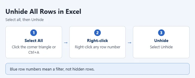
Excel only unhides rows inside your selection. That is why you select the whole sheet first. If you select a few rows, only the hidden rows between them come back.
Unhide All Rows From the Home Tab
Use the ribbon if right-clicking doesn’t show Unhide, or if you prefer menus.
- Click the Select All button, or press Ctrl+A.
- Select the Home tab.
- In the Cells group, select Format.
- Under Visibility, point to Hide & Unhide.
- Select Unhide Rows.
On Windows you can run the same command from the keyboard. Press Alt, then H, O, U, R, one key at a time.
Unhide All Rows With a Keyboard Shortcut
Select the whole sheet first, then press the shortcut for your version.
| Version | Select the whole sheet | Unhide rows |
|---|---|---|
| Excel for Windows | Ctrl+A | Ctrl+Shift+9 |
| Excel for Mac | Command+A | Shift+Command+( or Control+Shift+( |
| Excel for the web | Ctrl+A | Ctrl+Shift+9 |
The left parenthesis shares a key with 9, so the Mac shortcut uses the same keys as the Windows one. In Excel for the web, your browser may catch the shortcut before Excel does. If nothing happens, use the right-click method instead.
How to Unhide All Rows in Excel for Mac
- Click the Select All triangle in the top-left corner of the sheet, or press Command+A.
- Control-click any row number. You can also right-click or tap with two fingers on a trackpad.
- Select Unhide.
The ribbon path also works on a Mac. Go to Home > Format > Hide & Unhide > Unhide Rows.
How to Unhide All Rows in Excel for the Web
- Open the workbook in your browser and make sure you are in editing mode, not viewing mode.
- Click the Select All triangle in the top-left corner of the grid.
- Right-click any row number.
- Select Unhide Rows.
Menu labels in Excel for the web change more often than in the desktop apps. If you don’t see Unhide Rows, check that you right-clicked a row number and not a cell.
How to Unhide Specific Rows
Use this when you want some rows back and want others to stay hidden. It works the same way on Windows, Mac and the web.
- Find the gap in the row numbers. A double line between two row numbers marks hidden rows.
- Select the row above and the row below the gap. For example, if row 5 is hidden, drag across row numbers 4 and 6.
- Right-click the selection and select Unhide.
You can also double-click the double line between the two row numbers. The hidden rows open without any menu.
How to Unhide Row 1
Row 1 has no row above it, so you can’t select both sides of the gap. Select a cell in the hidden row by name instead.
- Click the Name Box to the left of the formula bar.
- Type A1 and press Enter. Cell A1 is now selected, even though you can’t see it.
- Select the Home tab, then select Format.
- Point to Hide & Unhide and select Unhide Rows.
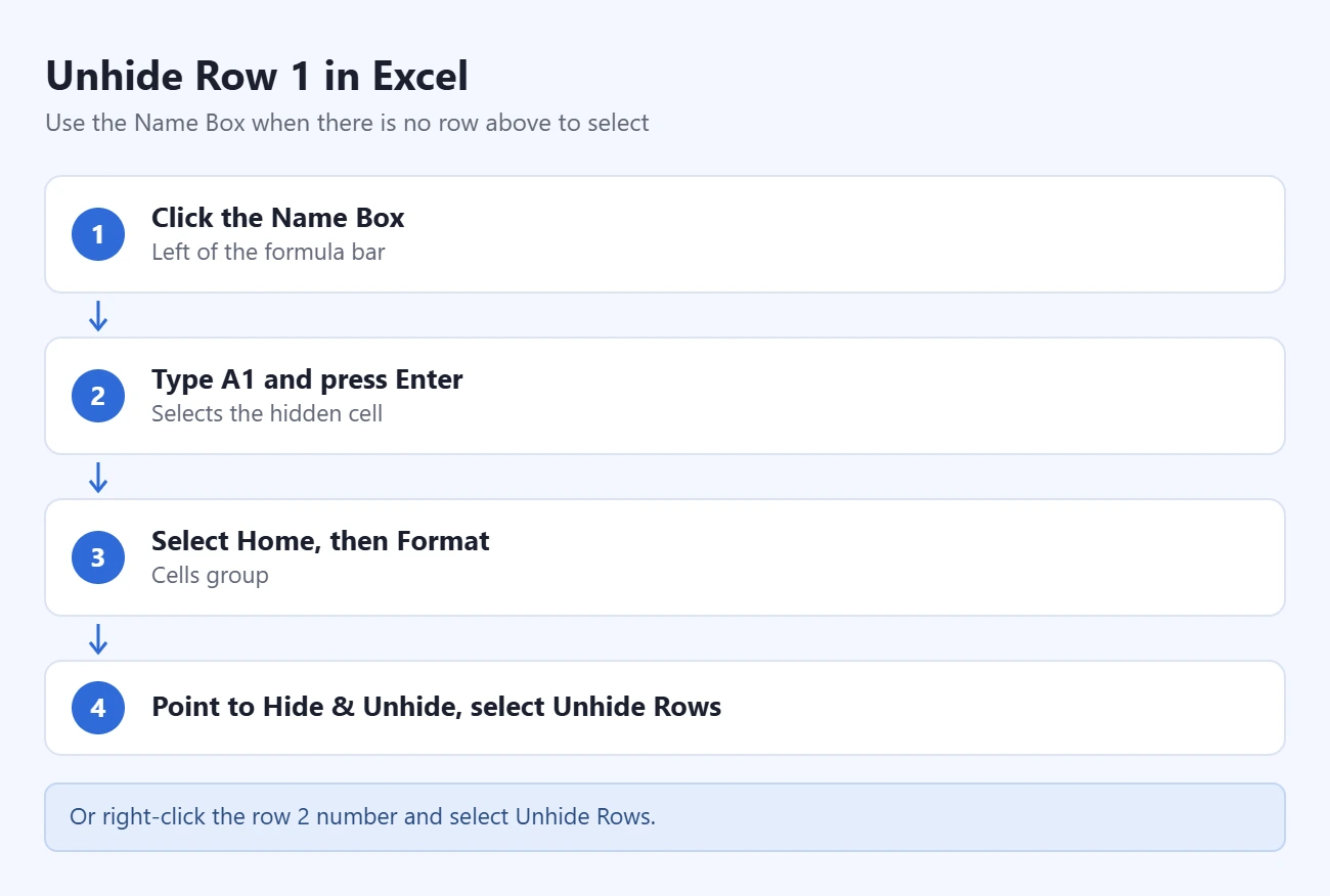
There is a quicker way when only row 1 is hidden. Right-click the row 2 number and select Unhide Rows. Microsoft covers both in its Unhide the first column or row in a worksheet guide. If several top rows are hidden, selecting the whole sheet and unhiding all rows brings them back too.
How to Confirm It Worked
Look at the row numbers on the left. They should count up with no skipped numbers and no double lines. Scroll to the top to check that row 1 is there.
If you unhid rows by mistake, press Ctrl+Z on Windows or the web, or Command+Z on a Mac. To hide rows again later, select them, right-click and select Hide.
Why Rows Might Still Be Missing
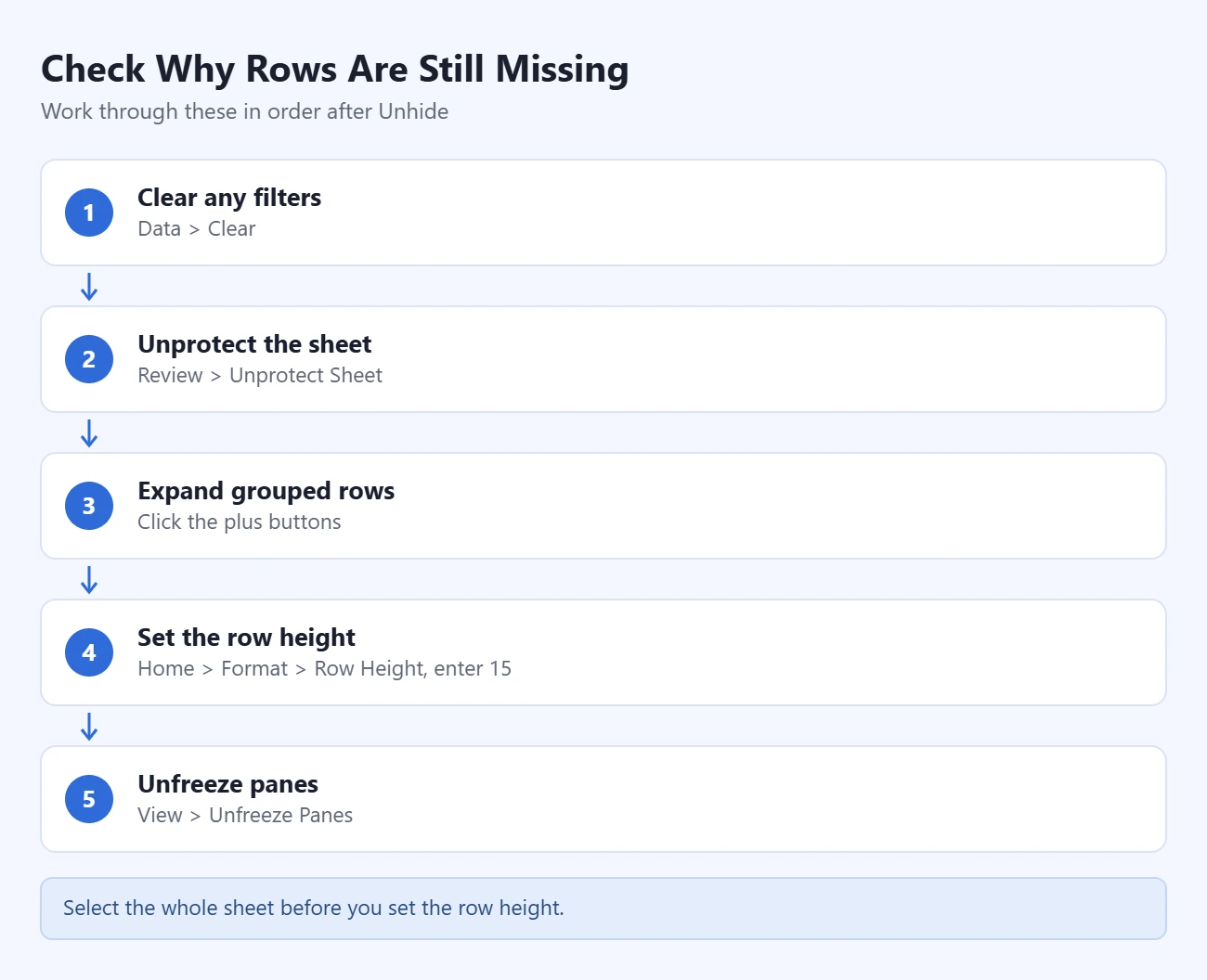
If row numbers still skip after you unhide everything, the rows are probably not hidden in the usual way. Work through these checks in order.
- Clear any filters. Go to the Data tab and select Clear.
- Unprotect the sheet. Go to the Review tab and select Unprotect Sheet.
- Expand grouped rows. Click the plus buttons to the left of the row numbers.
- Set the row height. Select the whole sheet, then go to Home > Format > Row Height and enter 15.
- Unfreeze panes. Go to the View tab and select Unfreeze Panes.
A filter is on
Filtered rows are not hidden rows, so Unhide ignores them. You can tell a filter is active when the row numbers are blue and a column header shows a filter icon instead of a plain arrow. Select Clear on the Data tab to show every row and keep the filter buttons. Select Filter on the same tab to turn filtering off completely.
The sheet is protected
On a protected sheet, Hide and Unhide are grayed out unless the person who protected it allowed row formatting. The Review tab shows Unprotect Sheet when protection is on. Select it and enter the password if you are asked. On Windows you can also go to File > Info > Protect > Unprotect Sheet. If you don’t know the password, ask the person who set it. Microsoft can’t recover it.
The rows are grouped
Plus and minus buttons in the left margin mean the sheet has an outline. Click a plus button to open one group, or click the highest number at the top of the margin to show every level. To remove the outline, go to Data > Ungroup > Clear Outline. Microsoft notes that rows can stay hidden if you remove an outline while a group is collapsed. If that happens, select the whole sheet and unhide the rows again.
The row height is zero or close to it
A row with a height of 0 is a hidden row, and Unhide brings it back. A row with a tiny height, such as 0.5, is different. It is too thin to see, but Excel doesn’t count it as hidden, so Unhide does nothing.
To fix it, select the whole sheet, or just the rows around the gap. Go to Home > Format > Row Height, type 15 and select OK. That is the default height in points for the standard font. You can also choose AutoFit Row Height from the same menu so each row fits its contents. For more on sizing, see how row and column sizing works in Excel.
Setting one height for the whole sheet replaces any custom row heights. If you sized some rows by hand, select only the rows around the gap.
Panes are frozen
If someone froze panes while the top rows were scrolled out of view, those rows can’t be reached by scrolling. They look hidden, but Unhide won’t change anything. Go to View > Unfreeze Panes, then scroll to the top. See how to freeze panes in Excel to set them up again in the right spot.
Only some rows came back
Your selection didn’t cover every hidden row. Click the Select All button so the entire sheet is highlighted, then select Unhide again.
Frequently Asked Questions
Is there a shortcut to unhide all rows in Excel?
Yes. Press Ctrl+A to select the whole sheet, then press Ctrl+Shift+9. On a Mac, press Command+A, then Shift+Command+(.
Why is Unhide grayed out in Excel?
The sheet is almost always protected. Go to the Review tab and select Unprotect Sheet, then try again. You need the password if the sheet has one.
How do I unhide all rows and columns at the same time?
Select the whole sheet. Right-click a row number and select Unhide, then right-click a column letter and select Unhide. Rows and columns are separate commands, so you need both.
How do I unhide columns instead?
Use the same steps, but right-click a column letter and select Unhide. The keyboard shortcut is Ctrl+Shift+0, but on Windows it can be taken over by the shortcut that switches keyboard languages. Use the right-click menu if it does nothing. To resize columns after, see how to AutoFit columns and rows in Excel.
Does unhiding rows change my data or formulas?
No. Hidden rows stay in the sheet the whole time, and formulas such as SUM keep counting them while they are hidden. Unhiding only makes them visible again.
Why do my rows hide again after I unhide them?
A filter, a collapsed group or a macro in the workbook is hiding them again. Clear the filters and expand the groups first. If the rows still disappear, ask the person who built the workbook whether it runs a macro.
How do I unhide rows in Google Sheets?
Google Sheets uses small arrows in the row numbers instead of an Unhide menu on the whole sheet. The steps for columns are in this guide on how to hide and unhide a column in Google Sheets, and rows work the same way.
Next Step
Once every row is visible, scroll through the sheet and check for data you didn’t know was there before you sort, print or share it. If you only wanted to keep headings in view, freezing the top row is a better choice than hiding the rows in between.

Matthew Burleigh has been writing tech tutorials since 2008. His writing has appeared on dozens of different websites and been read hundreds of millions of times.
After receiving his Bachelor’s and Master’s degrees in Computer Science he spent several years working in IT management for small businesses. However, he now works full time writing content online and creating websites.
His main writing topics include iPhones, Microsoft Office, Google Apps, Android, and Photoshop, but he has also written about many other tech topics as well.