How to Use VLOOKUP in Excel

To use VLOOKUP in Excel, type =VLOOKUP(lookup value, table range, column number, FALSE) and press Enter. For example, =VLOOKUP(E2,A2:C20,3,FALSE) finds the value in E2 in column A and returns the matching value from the third column. Use FALSE for an exact match. This guide covers Excel for Microsoft 365, Excel 2024, 2021, 2019 and 2016 on Windows and Mac.

The syntax, error causes and tips come from Microsoft’s VLOOKUP function page.

What You Need Before You Start

• Data arranged in columns. VLOOKUP searches down a column. If your data runs across rows, use HLOOKUP.
• The lookup value in the first column of the range. Microsoft says the value you look up must be in the first column of the range you select. The answer must be in a column to its right.
• Matching data types. If the first column holds numbers or dates stored as text, VLOOKUP can return a wrong or unexpected value.
• Clean values. Extra spaces before or after a value stop an exact match.

How to Write a VLOOKUP Formula

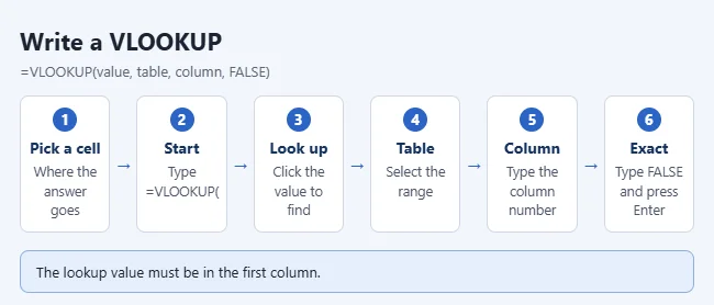
1. Click the cell where you want the result.
2. Type =VLOOKUP(. Excel shows a tip listing the four arguments.
3. Click the cell with the value you want to look up, such as a product ID, then type a comma.
4. Select the table to search. The lookup value must be in its first column. Type a comma.
5. Type the column number to return, counting from the left edge of the table you selected, then a comma. The first column is 1.
6. Type FALSE for an exact match, add a closing parenthesis, and press Enter. The cell shows the matching value.

What Each Part Means

The full syntax is =VLOOKUP(lookup_value, table_array, col_index_num, [range_lookup]).

• lookup_value: what you’re searching for. It can be a cell reference like E2, a number, or text in quotation marks like "P-103".
• table_array: the range to search. It must include both the column you search and the column that holds the answer.
• col_index_num: which column in that range holds the answer, starting with 1 for the leftmost column. It is not the worksheet column letter.
• range_lookup: FALSE (or 0) for an exact match. TRUE (or 1), or leaving it out, gives an approximate match and assumes the first column is sorted.

Leaving out the last argument is the most common mistake. The default is approximate match, so always type FALSE unless you want a band lookup.

A Complete Example: Look Up a Price by Product ID

Type this small table into cells A1 through C6 of a blank sheet.

Row	A	B	C
1	Product ID	Product	Price
2	P-101	Notebook	4.50
3	P-102	Desk lamp	18.00
4	P-103	USB cable	7.25
5	P-104	Stapler	9.99
6	P-105	Whiteboard	32.00

1. In cell E2, type P-103. This is the ID you want to find.
2. In cell F2, type =VLOOKUP(E2,A2:C6,3,FALSE) and press Enter.
3. F2 shows 7.25. Excel found P-103 in column A and returned the value from the third column of the range, which is Price.
4. Change the 3 to a 2, so the formula reads =VLOOKUP(E2,A2:C6,2,FALSE). F2 now shows USB cable.
5. Type a different ID in E2, such as P-105. The result updates on its own.

How to Copy a VLOOKUP Down a Column

When you copy a formula down, Excel shifts the cell references. The table range shifts too, and lower rows start to miss data. Lock the range first.

1. Click the cell with your formula and click inside the table range in the formula bar.
2. Press F4. The range changes to an absolute reference, such as $A$2:$C$6. You can also type the dollar signs yourself.
3. Press Enter. The formula should now read =VLOOKUP(E2,$A$2:$C$6,3,FALSE).
4. Drag the small square at the bottom-right corner of the cell down the column. E2 changes to E3, E4 and so on, while the table range stays put.

If your results come from a percentage or a total, the same dollar-sign rule applies. See how to calculate a percentage in Excel for more examples of absolute references.

Use the Function Arguments Box Instead of Typing

If you’d rather fill in labeled boxes, Excel for Windows has a guided dialog.

1. Click the cell where you want the result.
2. Click Insert Function (the fx button) on the formula bar. Excel adds the equals sign for you.
3. Type VLOOKUP in the Search for a function box, click Go, select VLOOKUP in the list, and click OK.
4. In the Function Arguments box, fill in the four fields: Lookup_value, Table_array, Col_index_num and Range_lookup. Type FALSE in the last one.
5. Click OK. The finished formula appears in the cell.

The layout of this tool differs in Excel for Mac and Excel for the web. Typing the formula works the same way everywhere.

Approximate Match: Look Up a Grade or Tax Band

Approximate match is for ranges of numbers, such as grade bands, tax brackets, shipping tiers or commission rates. Excel finds the largest value in the first column that is less than or equal to your lookup value.

Type this table into A1 through B6 of a new sheet. Each row is the lowest score for that grade.

Row	A	B
1	Minimum score	Grade
2	0	F
3	60	D
4	70	C
5	80	B
6	90	A

1. List the lowest value of each band. Put the minimums in the first column and the result next to each one.
2. Sort the first column smallest to largest. Approximate match gives wrong answers if it isn’t sorted.
3. Type the score to look up. Enter 84 in cell D2.
4. Enter the formula with TRUE. In E2, type =VLOOKUP(D2,$A$2:$B$6,2,TRUE) and press Enter.
5. Check the result. E2 shows B, because 80 is the largest minimum that is not above 84.

With the same table, a score of 59 returns F and a score of 90 returns A. A score below 0 returns #N/A, because it is smaller than the smallest value in the first column. A tax table works the same way: put the starting income of each bracket in the first column and the rate in the second.

Wildcards: Look Up Part of a Name

Microsoft says you can use wildcard characters in the lookup value when the last argument is FALSE and the lookup value is text.

• Asterisk (*) matches any number of characters.
• Question mark (?) matches exactly one character.
• Tilde (~) before a question mark or asterisk searches for that actual character.

These examples use the product table from earlier. Because the search is on the Product column, the range starts at column B.

• Begins with: =VLOOKUP("Desk*",B2:C6,2,FALSE) returns 18, the price of Desk lamp.
• Contains: =VLOOKUP("*cable*",B2:C6,2,FALSE) returns 7.25.
• One unknown character: =VLOOKUP("P-10?",A2:C6,2,FALSE) returns Notebook. All five IDs fit the pattern, and VLOOKUP returns the first one it finds.
• Text typed in a cell: =VLOOKUP(E2&"*",B2:C6,2,FALSE) looks for a product that starts with whatever is in E2.

A wildcard lookup returns only the first match, so make the pattern specific enough to fit one row.

Look Up Values on Another Sheet or in Another Workbook

The table doesn’t have to be on the same sheet as the formula.

Another sheet in the same workbook

1. Type =VLOOKUP(, click the lookup cell, and type a comma.
2. Click the tab of the sheet that holds the table.
3. Select the table range, then press F4 to lock it.
4. Type a comma, the column number, a comma, FALSE and a closing parenthesis. Press Enter.

Excel puts the sheet name and an exclamation point before the range, like =VLOOKUP(A2,Prices!$A$2:$C$6,3,FALSE). If the sheet name has a space or other nonalphabetical character, it goes in single quotation marks, like =VLOOKUP(A2,'Client Details'!A:F,3,FALSE).

Another workbook

1. Open both workbooks.
2. In the workbook where you want the result, type =VLOOKUP(, click the lookup cell, and type a comma.
3. Switch to the other workbook, click the sheet you need, and select the table range. Excel makes this reference absolute for you.
4. Type a comma, the column number, a comma, FALSE and a closing parenthesis. Press Enter. Excel takes you back to the first workbook.

While the source workbook is open, the formula looks like =VLOOKUP(A2,[Prices.xlsx]Sheet1!$A$2:$C$6,3,FALSE). After you close it, Excel adds the full folder path, like =VLOOKUP(A2,'C:\Reports\[Prices.xlsx]Sheet1'!$A$2:$C$6,3,FALSE). If you move or rename the source file, the link breaks and you need to point the formula at the new location.

Fix Common VLOOKUP Errors

• #N/A: With FALSE, the exact value wasn’t found. With TRUE, the lookup value is smaller than the smallest value in the first column.
• #REF!: The column number is bigger than the number of columns in your range. A three-column range can’t return column 4.
• #VALUE!: The column number is less than 1.
• #NAME?: Text in the formula is missing its quotation marks, or the function name is misspelled. Write "P-103", not P-103.
• #SPILL!: You used a whole column as the lookup value, like =VLOOKUP(A:A,A:C,2,FALSE). Point to one cell instead, or add an @ sign: =VLOOKUP(@A:A,A:C,2,FALSE).
• Wrong answer: You left out FALSE and the first column isn’t sorted.
• Right for the first row, wrong lower down: The table range wasn’t locked before you copied the formula. Add the dollar signs.

Work through a #N/A error

When you can see the value in the table but still get #N/A, check these in order.

1. Confirm the lookup column is first. The value must be in the leftmost column of the range you selected.
2. Check that the range covers the row. If it stops short or shifted when copied, lock it with F4.
3. Remove extra spaces. Use =VLOOKUP(TRIM(E2),$A$2:$C$6,3,FALSE), or clean the table column with TRIM.
4. Match the data types. A number stored as text will not match a real number. Convert one side so both are the same.
5. Show a message for values that are missing. Wrap the formula in IFNA, like =IFNA(VLOOKUP(E2,$A$2:$C$6,3,FALSE),"Not found").

IFNA only hides #N/A, so other errors still show and you can fix them. Use it after the formula works, not before.

VLOOKUP vs. XLOOKUP vs. INDEX and MATCH

All three find the price for the ID in E2 in the product table. Each returns 7.25 for P-103.

Function	Formula	Looks left?	Default match	Works in
VLOOKUP	=VLOOKUP(E2,A2:C6,3,FALSE)	No	Approximate	All versions covered here
XLOOKUP	=XLOOKUP(E2,A2:A6,C2:C6,"Not found")	Yes	Exact	Microsoft 365, Excel 2021 and 2024. Not Excel 2016 or 2019.
INDEX and MATCH	=INDEX(C2:C6,MATCH(E2,A2:A6,0))	Yes	Set by the 0 in MATCH	All versions covered here

• XLOOKUP takes a separate lookup range and return range, so there is no column number to count. It has a built-in “if not found” message. Microsoft describes it as an improved version of VLOOKUP that works in any direction.
• INDEX and MATCH does the same job in every version. MATCH finds the row and INDEX returns the value from that row. Microsoft suggests it when the lookup value isn’t in the first column.
• VLOOKUP still works in every Excel version covered here. Choose it when the file must open in Excel 2016 or 2019 and the lookup column is on the left.

To look left, such as finding the ID for Stapler, use =XLOOKUP("Stapler",B2:B6,A2:A6) or =INDEX(A2:A6,MATCH("Stapler",B2:B6,0)). Both return P-104.

One more difference matters in tables that change. VLOOKUP’s column number is a typed number, so inserting a column inside the table makes it point at the wrong column. The other two use ranges that move with the data.

Frequently Asked Questions

Should I use XLOOKUP instead?

If your version of Excel has it, Microsoft recommends XLOOKUP. It works in any direction and uses exact matches by default. It is not available in Excel 2016 or Excel 2019, so use VLOOKUP or INDEX and MATCH if anyone opening the file has those versions.

Can VLOOKUP look to the left?

No. It only returns values to the right of the lookup column. Use XLOOKUP or INDEX and MATCH, or rearrange your columns so the lookup column comes first.

Can VLOOKUP search another sheet?

Yes. Include the sheet name, like =VLOOKUP(A2,'Client Details'!A:F,3,FALSE). It can also search another workbook when the file name is in square brackets before the sheet name.

What happens if the lookup value appears more than once?

VLOOKUP returns the first match it finds from the top and ignores the rest. If repeats are a mistake, remove duplicates in Excel before you run the lookup.

Is VLOOKUP case-sensitive?

No. It treats uppercase and lowercase letters as the same, so p-103 and P-103 both match.

What’s the difference between TRUE and FALSE in VLOOKUP?

FALSE finds only an exact match and returns #N/A if there isn’t one. TRUE finds the closest value that is not larger than the lookup value and needs the first column sorted in ascending order. Leaving the argument out is the same as TRUE.

How do I stop people from typing IDs that don’t exist?

Let them pick from a list instead of typing. You can create a drop-down list in Excel that uses the first column of your lookup table as its source, so every choice has a match.

Next Step

Build the product table from the example, enter =VLOOKUP(E2,$A$2:$C$6,3,FALSE), and change the ID in E2 a few times. Once that works, swap in your own range and column number, and add IFNA to handle values that aren’t in the table.