To use COUNTIF in Excel, click an empty cell, type =COUNTIF(range, criteria), such as =COUNTIF(B2:B7,”East”), and press Enter. Excel returns how many cells in the range match that one condition. The function works the same way in Excel for Microsoft 365 on Windows and Mac, Excel 2024, Excel 2021, older desktop versions, and Excel for the web.
COUNTIF answers “how many” questions: how many orders came from the East region, how many sales were over $1,000, how many rows still have an empty Notes cell. It checks one condition. When you need two or more conditions at the same time, its sibling COUNTIFS takes over, and that’s covered further down along with the mistakes that make COUNTIF return 0 or an error.
The Two Parts of a COUNTIF Formula
Every COUNTIF formula has the same shape:
=COUNTIF(range, criteria)
- range is the group of cells Excel looks through, such as B2:B7 or a whole column like B:B. It can be a column, a row, a block of cells, or a named range.
- criteria is the test a cell has to pass to be counted. It can be a number (1200), text in quotes (“East”), a comparison in quotes (“>1000”), a cell reference (G2), or a pattern with wildcards (“A*”).
Both parts are required, and they’re separated by a comma. The result is always a single number. Microsoft’s COUNTIF function page describes the criteria argument the same way and notes that it accepts only one condition.
One rule covers most of the quoting confusion: text and anything with a comparison symbol goes inside double quotes, while plain numbers and cell references don’t need them. =COUNTIF(C2:C7,1200) and =COUNTIF(C2:C7,">1000") are both correct.
Sample Data Used in the Examples
Every formula below uses this small sales list. Type it into a blank sheet starting at cell A1 if you want to follow along and check each answer. Cells E3 and E6 are intentionally empty.
| Row | A: Rep | B: Region | C: Sales | D: Order Date | E: Notes |
|---|---|---|---|---|---|
| 2 | Alex | East | 1200 | 9/3/2026 | Rush |
| 3 | Priya | West | 850 | 9/15/2026 | |
| 4 | Jordan | east | 2400 | 10/2/2026 | Gift wrap |
| 5 | Sam | North | 450 | 10/9/2026 | Call first |
| 6 | Alex | West | 1750 | 10/20/2026 | |
| 7 | Taylor | East | 600 | 10/22/2026 | Rush |
Row 1 holds the headings (Rep, Region, Sales, Order Date, Notes). Leave the headings out of your range so they aren’t tested along with the data.
How to Write Your First COUNTIF Formula
This counts how many orders came from the East region.
- Click an empty cell outside the data, such as G2. Putting the formula inside the range it counts creates a circular reference.
- Type
=COUNTIF(. Excel shows a small tooltip with the two arguments as a reminder. - Drag over B2 through B7, or type
B2:B7. - Type a comma.
- Type
"East"with the double quotes. - Type the closing parenthesis, so the cell reads
=COUNTIF(B2:B7,"East"). - Press Enter (on a Mac, Return). The cell shows 3.
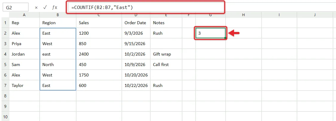
Why 3 and not 2? Jordan’s region was typed as lowercase “east”, and COUNTIF ignores letter case. “East”, “east” and “EAST” all count as the same value.
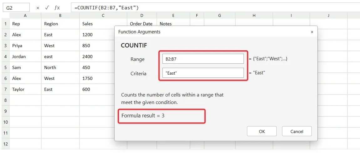
If you’d rather fill in boxes than type, Excel on Windows has a guided version. Click the result cell, go to Formulas > More Functions > Statistical > COUNTIF (or click the fx button next to the formula bar and search for COUNTIF). The Function Arguments window has a Range box and a Criteria box, and it previews the result before you click OK. On a Mac, Formulas > Insert Function opens the Formula Builder pane, which works the same way.
Count Cells That Match Specific Text
Exact text matches are the most common use. A few examples from the sample list:
| Goal | Formula | Result |
|---|---|---|
| Orders by Alex | =COUNTIF(A2:A7,"Alex") | 2 |
| Orders from West | =COUNTIF(B2:B7,"West") | 2 |
| Orders not from East | =COUNTIF(B2:B7,"<>East") | 3 |
| Notes that say exactly Rush | =COUNTIF(E2:E7,"Rush") | 2 |
An exact match means the whole cell has to equal the text. A cell that says “Rush order” would not be counted by "Rush". For “contains” style matches, use the wildcards described a little later.
The <> symbol means “not equal to.” Be aware that “not equal to East” also counts empty cells, since an empty cell isn’t East. If your range has gaps, the “not equal” count will be higher than the number of filled cells that differ.
Count Numbers Above, Below, or Equal to a Value
For numbers, put the comparison symbol and the number together inside one pair of quotes. Excel supports six operators:
| Operator | Meaning | Example | Result |
|---|---|---|---|
| = | Equal to | =COUNTIF(C2:C7,1200) | 1 |
| > | Greater than | =COUNTIF(C2:C7,">1000") | 3 |
| < | Less than | =COUNTIF(C2:C7,"<500") | 1 |
| >= | Greater than or equal to | =COUNTIF(C2:C7,">=850") | 4 |
| <= | Less than or equal to | =COUNTIF(C2:C7,"<=600") | 2 |
| <> | Not equal to | =COUNTIF(C2:C7,"<>600") | 5 |
Pay attention to the difference between > and >=. A target of exactly 850 is counted by ">=850" but not by ">850", and that single character is the usual reason a count is off by one.
Counting values between two numbers
COUNTIF can’t hold “between” in one condition, but you can subtract one count from another. To count sales from 600 through 1,500:
=COUNTIF(C2:C7,">=600")-COUNTIF(C2:C7,">1500")
The first part counts 5 sales of 600 or more, the second removes the 2 that are over 1,500, and the answer is 3 (1200, 850 and 600). The COUNTIFS version later in this guide does the same thing in a way that’s easier to read.
Use a Cell Reference as the Condition
Typing the condition into a cell instead of the formula lets you change the count without editing anything. Put West in cell G5, then use:
=COUNTIF(B2:B7,G5)
The result is 2. Type East in G5 and it changes to 3. Notice there are no quotes around G5. Quotes would make Excel look for the literal letters “G5”.
Comparisons need one extra piece. Say G6 holds the number 1000 and you want sales above it. Keep the operator in quotes and join it to the cell with an ampersand (&):
=COUNTIF(C2:C7,">"&G6)
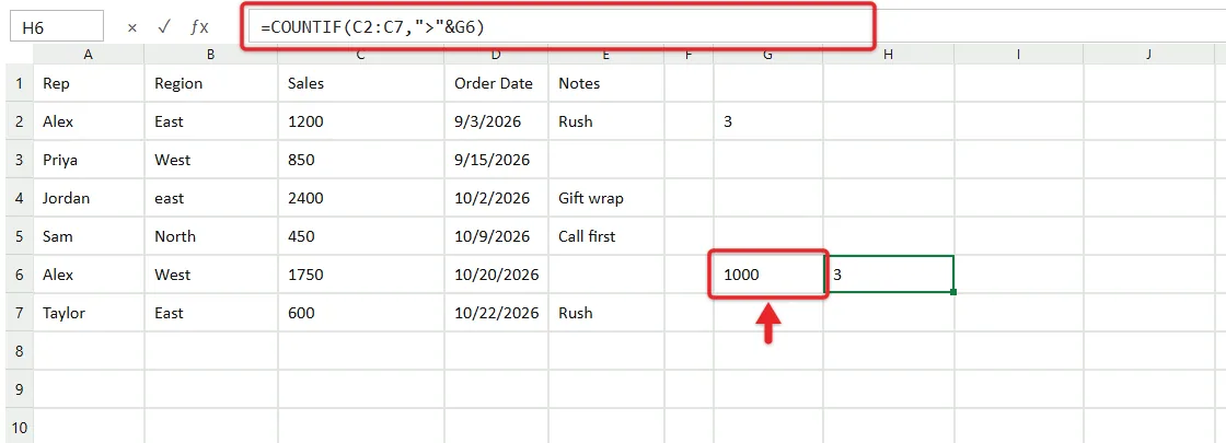
That returns 3. Writing ">G6" all inside the quotes is a common slip. Excel then compares against the text “G6” instead of the number 1000 and returns 0.
If you plan to copy the formula to other cells, lock the range with dollar signs, such as $B$2:$B$7. Otherwise the range shifts as you fill down and the counts drift.
Count Dates Before, After, or Within a Period
Excel stores each date as a serial number, so date conditions work like number conditions. The safest way to write a date into the criteria is the DATE function, which reads year, month and day in that order no matter what date format your computer uses:
| Goal | Formula | Result |
|---|---|---|
| Orders on or after October 1, 2026 | =COUNTIF(D2:D7,">="&DATE(2026,10,1)) | 4 |
| Orders before October 1, 2026 | =COUNTIF(D2:D7,"<"&DATE(2026,10,1)) | 2 |
| Orders on one exact date | =COUNTIF(D2:D7,DATE(2026,10,20)) | 1 |
| Orders dated today or later | =COUNTIF(D2:D7,">="&TODAY()) | Changes daily |
You can also type a date in quotes, like ">10/1/2026", and on a US-format computer it works. The DATE version is more dependable if the file is opened on a computer set to day-first dates, where 10/1 means January 10.
Dates typed as text (often the case after pasting from a website or another program) won’t be counted by any of these formulas. If a date sits on the left edge of its cell instead of the right, it’s probably text.
Match Part of a Cell With Wildcards
Wildcards turn an exact match into a pattern. COUNTIF understands three characters:
- * (asterisk) stands for any number of characters, including none.
- ? (question mark) stands for exactly one character.
- ~ (tilde) placed before * or ? tells Excel to look for an actual asterisk or question mark.
| Goal | Formula | Result |
|---|---|---|
| Reps whose name starts with A | =COUNTIF(A2:A7,"A*") | 2 |
| Reps whose name ends in r | =COUNTIF(A2:A7,"*r") | 1 |
| Notes containing “wrap” anywhere | =COUNTIF(E2:E7,"*wrap*") | 1 |
| Names exactly four letters long | =COUNTIF(A2:A7,"????") | 2 |
| Any cell containing text | =COUNTIF(E2:E7,"*") | 4 |
| Cells containing a real asterisk | =COUNTIF(E2:E7,"*~**") | 0 |
To combine a wildcard with a cell, join them the same way as an operator: =COUNTIF(E2:E7,"*"&G7&"*") counts notes that contain whatever word is typed in G7.
Wildcards only apply to text. A criteria of "1*" won’t count the number 1200, because it’s stored as a number rather than as the characters 1, 2, 0, 0.
Count Blank and Non-Blank Cells
Two short criteria handle empty cells in the Notes column:
=COUNTIF(E2:E7,"")counts empty cells and returns 2.=COUNTIF(E2:E7,"<>")counts cells that aren’t empty and returns 4.
These are handy for progress checks, such as how many rows still need a note. Excel also has dedicated functions for the same job, which the comparison section below explains. Watch out for cells that look empty but hold a space. They count as filled, and =COUNTIF(E2:E7," ") (a space between the quotes) will reveal how many there are.
Uppercase and Lowercase Are Treated the Same
Microsoft documents that COUNTIF criteria aren’t case sensitive, which is why East and east were counted together in the first example. Most of the time that’s what you want. If you need a case-sensitive count, COUNTIF can’t do it, but the EXACT function can, wrapped in SUMPRODUCT:
=SUMPRODUCT(--EXACT(B2:B7,"East"))
EXACT returns TRUE only where the capitalization matches, the two minus signs turn TRUE and FALSE into 1 and 0, and SUMPRODUCT adds them up. With the sample data this returns 2, leaving out Jordan’s lowercase entry.
The 255-Character Limit on Long Text
COUNTIF gives incorrect results when the text you’re matching is longer than 255 characters. That rarely matters for names or categories, but it can come up with product descriptions, survey comments, or URLs.
Microsoft’s suggested fix is to split the long text into pieces and join them with the & operator or CONCATENATE, for example =COUNTIF(A2:A100,"first part of the text"&"second part of the text"). When the long text already sits in a cell, a formula that avoids COUNTIF entirely is often simpler:
=SUMPRODUCT(--(A2:A100=G8))
That compares every cell to G8 with a plain equals test, which has no 255-character cap. Like COUNTIF, the equals sign ignores case. It does not understand wildcards, though.
Count With More Than One Condition Using COUNTIFS
COUNTIFS counts rows where every condition is true at once. You give it pairs of a range and a condition:
=COUNTIFS(criteria_range1, criteria1, criteria_range2, criteria2, ...)
To count East orders over $1,000:
=COUNTIFS(B2:B7,"East",C2:C7,">1000")
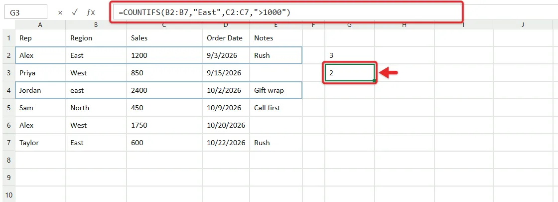
The result is 2: Alex’s 1,200 and Jordan’s 2,400. Taylor is in East too, but 600 fails the second test. Other useful patterns:
- Between two values:
=COUNTIFS(C2:C7,">=600",C2:C7,"<=1500")returns 3. Using the same range twice is allowed. - Dates in one month:
=COUNTIFS(D2:D7,">="&DATE(2026,10,1),D2:D7,"<"&DATE(2026,11,1))returns 4 October orders. - Text plus a blank check:
=COUNTIFS(B2:B7,"West",E2:E7,"")returns 2, the West orders with no note.
According to Microsoft’s COUNTIFS function page, you can use up to 127 range and condition pairs, and every range must have the same number of rows and columns as the first one. Mismatched sizes, such as B2:B7 with C2:C10, produce a #VALUE! error. The same page notes that a condition pointing at an empty cell is treated as 0, so an empty G-cell can quietly change your count.
Count Either of Two Values (OR Logic)
COUNTIFS only does “and.” To count rows that match one value or another, add two COUNTIF formulas together:
=COUNTIF(B2:B7,"East")+COUNTIF(B2:B7,"West")
That returns 5 (3 East plus 2 West). A shorter version puts the choices in curly braces and wraps the result in SUM:
=SUM(COUNTIF(B2:B7,{"East","West"}))
Adding counts works cleanly when one cell can’t match both options, as with a single region per row. If the conditions could overlap, such as notes that contain “Rush” or contain “wrap,” a cell holding both words would be counted twice. In that case subtract the overlap with a COUNTIF that tests for both, or use a helper column.
COUNTIF vs. COUNT, COUNTA, and COUNTBLANK
Excel has several counting functions, and picking the right one saves writing criteria you don’t need:
| Function | What it counts | Sample formula | Result |
|---|---|---|---|
| COUNT | Cells that contain numbers (dates count as numbers) | =COUNT(C2:C7) | 6 |
| COUNTA | Cells that aren’t empty, of any type | =COUNTA(E2:E7) | 4 |
| COUNTBLANK | Empty cells | =COUNTBLANK(E2:E7) | 2 |
| COUNTIF | Cells that meet one condition you choose | =COUNTIF(B2:B7,"East") | 3 |
| COUNTIFS | Rows that meet all of several conditions | =COUNTIFS(B2:B7,"East",C2:C7,">1000") | 2 |
One subtle difference: Microsoft’s COUNTBLANK page says it also counts cells whose formula returns empty text (“”), while a cell holding 0 isn’t blank. COUNTA treats those same formula cells as filled, because a formula is there. If your column is full of IF formulas that show nothing, COUNTBLANK will give the more intuitive answer.
COUNTIF looks only at what’s in a cell, never its formatting, so it can’t count by fill color. Counting the condition that produced the color usually works, and the guide to counting colored cells in Excel covers the filter and VBA alternatives for colors applied by hand.
Practical Uses Beyond a Single Total
COUNTIF becomes more useful once it’s paired with other features:
- Spot duplicates. In F2, enter
=COUNTIF($A$2:$A$7,A2)and fill down. Any row showing 2 or more is a repeat, so both of Alex’s rows show 2. When you’re ready to delete the extras, see how to remove duplicates in Excel. - Highlight repeats. The same idea works as a rule.
=COUNTIF($A$2:$A$7,A2)>1in a formula-based rule colors every repeated name, as shown in the guide to conditional formatting in Excel. - Build a summary. List each region in G10:G12 and enter
=COUNTIF($B$2:$B$7,G10)next to the first one, then fill down for a quick tally per region. - Share of the total.
=COUNTIF(B2:B7,"East")/COUNTA(B2:B7)formatted as a percentage shows that 50% of orders came from East.
When you need the dollar amount of those orders instead of how many there are, SUMIF uses the same range and criteria pattern with a third argument for the numbers to add. The guide on how to sum a column in Excel covers SUM, SUMIF and totals for filtered lists.
Using COUNTIF in Excel for the Web and on a Mac
The formula itself is identical everywhere. Type =COUNTIF(B2:B7,"East") into a cell in Excel for the web, Excel for Mac, or the desktop app on Windows and you get the same 3. A few things differ around it:
- Excel for the web: type the formula directly, or click the fx button by the formula bar to search for the function and fill in its arguments. Keeping the data you’re counting in the same workbook avoids the closed-workbook problem described in the errors section.
- Excel for Mac: press Return to finish a formula. Formulas > Insert Function opens the Formula Builder pane on the right side of the window instead of a pop-up box.
- Older desktop versions: COUNTIF and COUNTIFS have been in Excel for many years, so they work in Excel 2016 and 2019 too. The SUM and curly-brace OR shortcut and the SUMPRODUCT formulas in this guide also work there with a normal Enter.
When COUNTIF Returns 0, the Wrong Number, or an Error
The result is 0 but you can see matches
- Extra spaces or hidden characters. “East ” with a trailing space doesn’t equal “East”. Microsoft recommends cleaning imported text with TRIM or CLEAN. A quick check is
=COUNTIF(B2:B7,"*East*"); if that finds more matches than"East", stray characters are the cause. - Numbers stored as text. Numbers pasted from other programs are sometimes text. Comparisons such as
">1000"skip them. Look for a small green triangle in the corner of the cell, click the warning icon, and choose Convert to Number. - The operator and cell reference are both inside the quotes. Change
">G6"to">"&G6. - Curly quotes. Formulas copied from a document or email can carry curly quotation marks. Retype them as straight quotes in Excel.
The formula shows as text instead of a number
If the cell displays =COUNTIF(B2:B7,"East") rather than 3, the cell was formatted as Text before you typed. Change the format to General on the Home tab, then click into the cell, press F2, and press Enter. Also check that the formula starts with an equals sign and not a space.
#VALUE! error
Microsoft notes that COUNTIF returns #VALUE! when it refers to cells in another workbook that’s closed. Open the other workbook and the count calculates again. With COUNTIFS, #VALUE! usually means the ranges are different sizes.
#NAME? error
The function name is misspelled (COUNTIFF and COUTIF are common) or a text value is missing its quotes, so Excel reads East as a name it doesn’t know. Fix the spelling or add the quotes.
The count is too high or too low by a little
Check whether you meant > or >=, whether the heading row is inside the range, and whether “not equal” is picking up blank cells. For text over 255 characters, use the workaround in that section above.
Common COUNTIF Questions
Can COUNTIF look at more than one column?
Yes, if the same test applies to every cell. =COUNTIF(A2:E7,"Rush") searches the whole block and counts each matching cell. If you need a different condition for each column, use COUNTIFS instead.
Does COUNTIF count cells on another sheet?
It does. Include the sheet name and an exclamation point before the range, such as =COUNTIF(Orders!B2:B500,"East"). Wrap names with spaces in single quotes: ='Q4 Orders'!B2:B500. Clicking the other sheet while typing the formula fills this in for you.
Can I use a whole column like B:B?
You can, and it saves updating the formula when rows are added. Just keep the formula itself out of that column, and remember the heading in row 1 will be tested too. That rarely matters for numbers, but a heading like “East Sales” could match a wildcard search.
How do I count TRUE or FALSE values?
Use the logical value without quotes: =COUNTIF(F2:F50,TRUE). This is common with checkbox columns, where a checked box stores TRUE.
Is COUNTIF the same in Google Sheets?
The syntax, operators and wildcards match, so the formulas in this guide work in Google Sheets as well. Menus for inserting functions are different, but typing the formula directly works the same way.
Start with one of the formulas above on your own data, then swap the hard-typed condition for a cell reference. Once that works, COUNTIFS is the natural next step for reports that need two or three conditions at once.

Matthew Burleigh is the founder, head writer, and editor of Solve Your Tech, which he launched in 2012. He has written technology tutorials since 2008 and worked in IT since 2003, including small-business support, IT management, and consulting. He holds Bachelor’s and Master’s degrees in Computer Science from Arizona State University.
Matthew writes practical guides for Windows, iPhone and iPad, Microsoft Office, Outlook, Google apps, and Android. Solve Your Tech’s guides are checked step by step against the device or app maker’s own documentation and tested on his own devices whenever he has the hardware or software, with clear steps, sources, and update dates.
Read more about Matthew and how Solve Your Tech writes and updates its guides, or report a correction.