You add a new row to the bottom of a sales list, and the total at the bottom of the sheet doesn’t budge. The formula in the last column is blank on the new row because nobody copied it down. None of that is your fault. It happens because a plain range of cells has no idea where your data begins or ends.
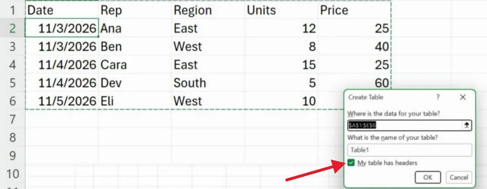
The fix is one shortcut. Click inside your data, press Ctrl+T, confirm that your table has headers, and Excel turns the range into a real table. From then on the table grows when you add rows, formulas fill down on their own, every header gets a sort and filter button, and you can total any column with a checkbox. It takes about three seconds, and it removes most of the small chores that make spreadsheets tedious.
The Range Grows When Your Data Does
Here is the sample data used throughout this article. Say it starts as a plain range in A1:E5.
| Date | Rep | Region | Units | Price |
|---|---|---|---|---|
| 11/3 | Ana | East | 12 | 25 |
| 11/3 | Ben | West | 8 | 40 |
| 11/4 | Cara | East | 15 | 25 |
| 11/4 | Dev | South | 5 | 60 |
Once it’s a table, typing in the first empty row underneath is all it takes to extend it. Microsoft’s own description is plain: start typing in a cell below the last table row and the table expands to include the new row. Pasting works the same way if you paste into the leftmost cell below the table. The banded shading, the filter buttons, and every formula that points at the table come along automatically. You never have to edit a range address from A2:E5 to A2:E6 again.
Formulas Read Like Sentences
Excel names a new table Table1, Table2, and so on. Rename it in the Table Name box on the Table Design tab. Call this one Sales. Now formulas can use the table and column names instead of cell addresses, which Microsoft calls structured references.
=SUM(Sales[Units])adds the Units column. With the four rows above, it returns 40.=AVERAGE(Sales[Price])returns 37.5.[@Units]means “the Units value in this same row,” which is how formulas inside the table refer to their neighbors.
The real payoff is that these references adjust whenever you add or remove data. Add a fifth row for Eli in the West region with 10 units at 40, and =SUM(Sales[Units]) immediately returns 50 without anyone touching the formula. Six months from now, anyone reading Sales[Units] also knows exactly what it adds, which is not true of D2:D5.
Type a Formula Once and the Whole Column Fills
Add a header called Total in F1, which makes F a new table column. In F2, type =[@Units]*[@Price] and press Enter. Excel fills that formula into every row of the column. This is a calculated column, and it stays consistent: change the formula in one cell and the change spreads to the whole column.
| Rep | Units | Price | Total |
|---|---|---|---|
| Ana | 12 | 25 | 300 |
| Ben | 8 | 40 | 320 |
| Cara | 15 | 25 | 375 |
| Dev | 5 | 60 | 300 |
| Eli | 10 | 40 | 400 |
No fill handle, no double-clicking the corner of a cell, no rows halfway down the sheet where someone forgot to copy the formula. Eli’s row picked up its 400 the moment it joined the table.
A Total Row That Respects Your Filters
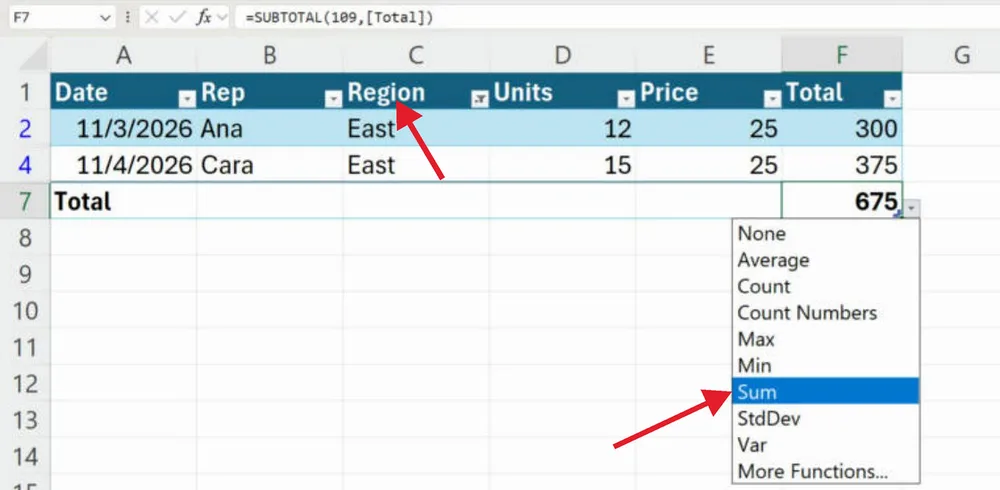
Click anywhere in the table, go to Table Design, and check Total Row. A row appears at the bottom, and each cell in it has a drop-down where you can pick Sum, Average, and other functions. Choose Sum under Total and you get 1,695 for the five rows above (300 + 320 + 375 + 300 + 400).
Look at the formula Excel wrote, though. It isn’t a plain SUM. It’s =SUBTOTAL(109,[Total]), and SUBTOTAL ignores rows that a filter has hidden. Use the Region header’s filter button to show only East, and the total drops to 675 (Ana’s 300 plus Cara’s 375). Clear the filter and it goes back to 1,695. That makes the Total Row a quick way to answer “how much did this region sell” without writing a SUMIF.
Filters, Banding, and Slicers Come Built In
Every header in a table gets a filter button by default, so sorting by Units or showing only one rep is two clicks away. If you want more on that, see this guide to making sortable headings in Excel. Banded rows shade every other line, so your eye doesn’t drift into the wrong row on a wide sheet.
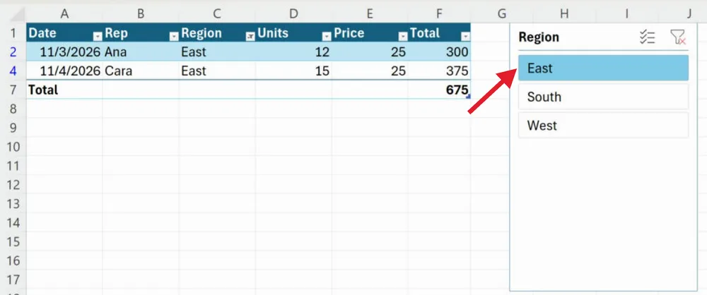
For something more visual, click in the table and choose Insert, then Slicer. Check Region and click OK. You get a panel with East, West, and South buttons that filter the table with one click. It’s a friendlier way to hand a filtered view to someone who doesn’t want to poke at drop-down arrows.
Everything Built on Top Stays in Sync
A table makes a better foundation for the other tools you already use. Microsoft recommends formatting data as a table before you build a PivotTable from it, and when you add rows, you refresh the PivotTable (Alt+F5 refreshes the selected one). Our pivot table guide for Excel walks through building one from scratch.
Drop-down lists benefit too. If the list of options for a data validation drop-down lives in a table, Microsoft notes that any drop-downs based on that table update automatically as you add or remove items. Add a new region to a Regions table and it shows up in every drop-down that uses it. Rules like conditional formatting in Excel are easier to manage on a table, too, since the data you’re highlighting has a fixed, named home.
Where Tables Work and What They Won’t Do
| Item | Details |
|---|---|
| Excel versions | Excel for Microsoft 365 (Windows and Mac), Excel for the web, and Excel 2024, 2021, 2019, and 2016 |
| Create a table | Ctrl+T, or Insert, then Table |
| Restyle a table | Home, then Format as Table |
| Subtotals command | Not available inside a table (use the Total Row or convert to a range) |
| PivotTables | Still need a refresh after you add data |
| Undo it | Table Design, then Convert to Range |
Two other cautions. If you leave “My table has headers” unchecked, Excel inserts its own Column1, Column2 header row and pushes your data down a row. And if you convert a table back to a range, the styling stays, but the filter buttons go away and structured references in your formulas turn into regular cell references.
How to Turn Your Data Into a Table
- Clean up first: make sure the data has one header row and no completely blank rows in the middle. If you have repeats, remove duplicates in Excel before you start.
- Click any cell inside the data.
- Press Ctrl+T (or choose Insert, then Table).
- Confirm the range, check My table has headers, and click OK.
- On the Table Design tab, type a short name like Sales in the Table Name box.
Microsoft’s create a table page covers the same steps for Windows, Mac, and the web.
Quick Answers About Excel Tables
Is an Excel table the same as a data table?
No. The data tables in Excel’s what-if analysis tools are a different feature. The tables in this article are what Excel used to call lists.
Can I have more than one table on a sheet?
Yes. You can create as many tables as you want in a spreadsheet, and each one gets its own name.
Will converting to a table change my existing formatting?
Excel applies a table style when it creates the table. You can pick a different look from Home, then Format as Table, and if you later convert back to a range, the style formatting stays in place.
Start with the list you update most often, the one where you’re always stretching a SUM range or copying a formula down. Press Ctrl+T, name the table, turn on the Total Row, and add your next entry underneath. Watching the total change on its own is usually enough to make you do the same thing to every other list you own.

Matthew Burleigh is the founder, head writer, and editor of Solve Your Tech, which he launched in 2012. He has written technology tutorials since 2008 and worked in IT since 2003, including small-business support, IT management, and consulting. He holds Bachelor’s and Master’s degrees in Computer Science from Arizona State University.
Matthew writes practical guides for Windows, iPhone and iPad, Microsoft Office, Outlook, Google apps, and Android. Solve Your Tech’s guides are checked step by step against the device or app maker’s own documentation and tested on his own devices whenever he has the hardware or software, with clear steps, sources, and update dates.
Read more about Matthew and how Solve Your Tech writes and updates its guides, or report a correction.