How to Insert Sparklines in Excel

To insert sparklines in Excel, select the empty cell at the end of a row of numbers, go to Insert, pick Line, Column or Win/Loss in the Sparklines group, select the row’s numbers as the Data Range, and select OK. Drag the fill handle down to give each row its own.

Picture a sales sheet with monthly figures per region and a small trend line beside each row. That’s what sparklines do in Excel for Microsoft 365, 2024, 2021, 2019 and 2016.

What a Sparkline Is

A sparkline is a miniature chart drawn inside a single cell. Unlike a regular chart, it isn’t a floating object you have to move around. It sits in the cell, resizes with the cell, and redraws when the numbers change.

Excel offers three kinds:

• Line shows the shape of a trend over time, such as monthly sales.
• Column shows each value as a small bar, which makes individual months easier to compare.
• Win/Loss ignores size and only shows whether each value is positive or negative.

Add a Sparkline to One Row

Here’s a sample layout. Marcus tracks sales for three regions, with January through June in columns B to G and an empty column H for the trend.

Region	Jan	Feb	Mar	Apr	May	Jun	Trend
North	4200	4500	4100	4800	5200	5600	(sparkline)
South	3900	3700	3500	3600	3300	3100	(sparkline)
West	2800	3400	2900	3500	3000	3600	(sparkline)

1. Click cell H2, the empty cell at the end of the North row.
2. Select the Insert tab.
3. In the Sparklines group, select Line. The Create Sparklines dialog opens with H2 already in the Location Range box.
4. Click in the Data Range box and drag across B2:G2, or type B2:G2.
5. Select OK.

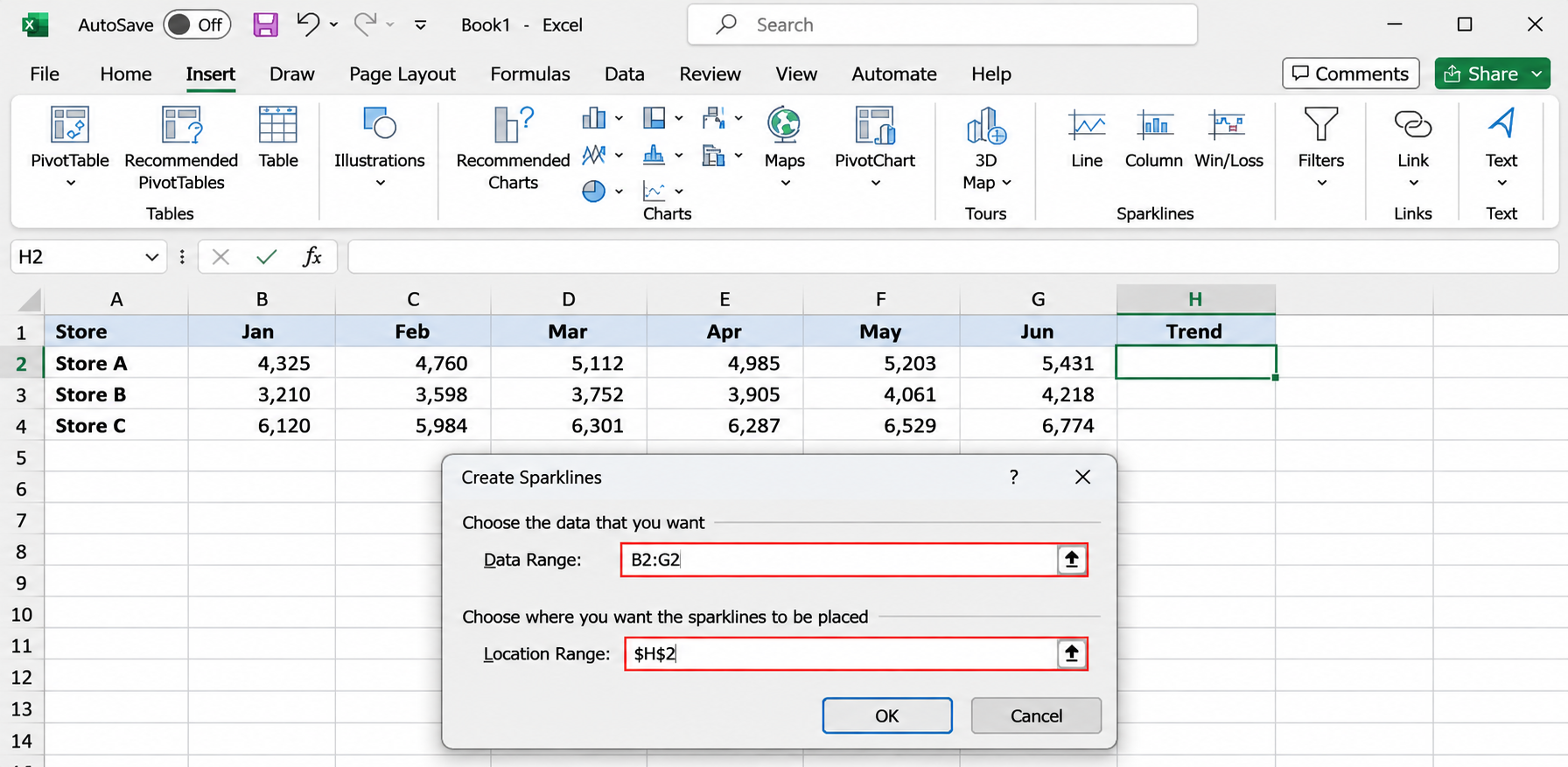
A small line appears in H2, rising from left to right. Widen column H and make row 2 a little taller if the line looks cramped. A sparkline stretches to fill whatever size the cell is.

Fill the Rest of the Rows

You have three ways to give each row a sparkline.

Drag the fill handle. Select H2, then drag the small square at the bottom right corner of the cell down to H4. Excel adjusts the data range for each row, just as it does with a formula.

Fill Down. Select H2:H4 and press Ctrl+D.

Create them all at once. Select B2:G4 first, choose Insert > Line, and type H2:H4 in the Location Range box. The location range has to match the shape of the data: three rows of data need three cells in a column. If the sizes don’t match, Excel warns you that the range isn’t valid.

Sparklines made together, or by filling, form a group. Click any one of them and Excel outlines the whole set. Formatting changes apply to every sparkline in the group, which keeps the column consistent.

Sparklines can sit beside a PivotTable too, but check their data range after you change the PivotTable layout, because the range doesn’t move with it.

Another shortcut on Windows is Quick Analysis. Select B2:G4, click the Quick Analysis button that appears at the bottom right of the selection (or press Ctrl+Q), open the Sparklines tab, and choose a type. Excel places the sparklines in the next empty column.

Line, Column or Win/Loss: Which to Pick

If you want to show	Pick	Example
The overall direction across many periods	Line	Twelve months of revenue
Which period was biggest or smallest	Column	Weekly sign-ups for a quarter
Hit or miss, profit or loss, win or lose	Win/Loss	Months above or below budget

Win/Loss works best with data that is already positive or negative. For a simple record, type 1 for a hit and -1 for a miss. A budget sheet can feed it a difference formula, such as actual minus budget, so months over budget show above the line and months under it show below.

You can switch types later. Select a sparkline, go to the Sparkline tab, and choose Line, Column or Win/Loss.

Format Sparklines

When you select a sparkline cell, a contextual tab appears on the ribbon. Microsoft’s page calls it the Sparkline tab, and some versions label it Sparkline Design or Sparkline Tools. It holds every formatting option:

• Show check boxes: High Point, Low Point, Negative Points, First Point, Last Point and Markers. Markers (Line only) put a dot on every value. High Point and Low Point are usually the most useful, because they point the reader straight at the best and worst month.
• Style: a gallery of preset color combinations.
• Sparkline Color: the line or bar color, plus Weight for line thickness.
• Marker Color: separate colors for markers and for the high, low, first, last and negative points.

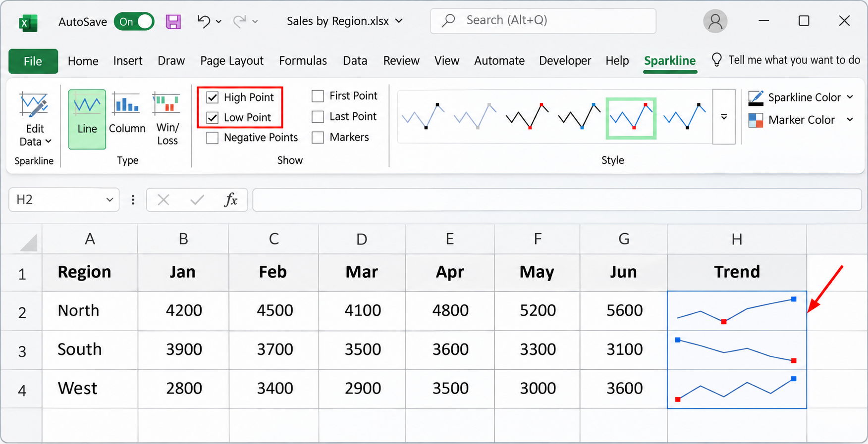
Keep it light. A thin dark line with red low points and green high points reads well at small sizes. Shading every marker in a different color turns a tiny chart into noise.

Make Rows Comparable With the Axis Settings

Here’s the surprise that trips most people up. By default, each sparkline scales itself to its own lowest and highest values. In Marcus’s sheet, the South line drops from 3,900 to 3,100 and the North line climbs from 4,200 to 5,600, yet both lines fill the full cell height. They look equally dramatic even though the North numbers are larger.

To compare rows fairly, put them on the same scale:

1. Select any sparkline in the group.
2. On the Sparkline tab, select Axis.
3. Under Vertical Axis Minimum Value Options, choose Same for All Sparklines.
4. Select Axis again and choose Same for All Sparklines under Vertical Axis Maximum Value Options.

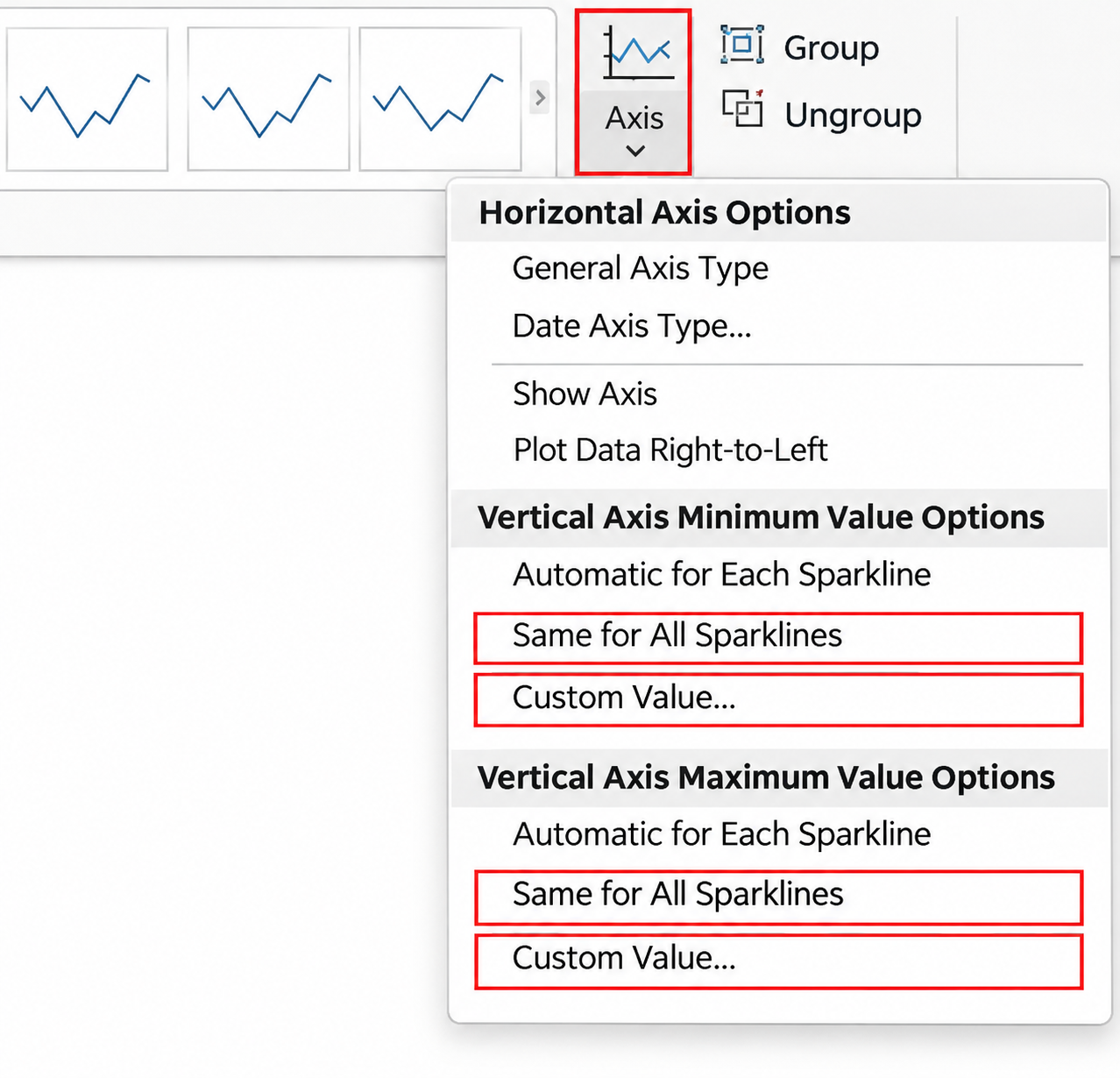
Now a taller line really means a larger number. For a fixed scale, choose Custom Value instead and type a minimum such as 0. Don’t force a minimum of 0 when the data has negative values, because anything below the minimum is cut off.

The Axis menu has two more choices. Show Axis draws a horizontal line at zero, which only appears when the data crosses zero. Date Axis Type spaces points by actual dates when the periods are uneven, such as readings taken on irregular days.

Handle Blank and Hidden Cells

A missing month can break a line in a confusing way. Select a sparkline, go to Edit Data on the Sparkline tab, and choose Hidden & Empty Cells. You’ll get three choices for empty cells:

• Gaps leaves a break in the line, which is honest when data is missing.
• Zero drops the line to zero, which suits months with genuinely no sales.
• Connect data points with line bridges the gap.

The same dialog has Show data in hidden rows and columns. Leave it off if you hide columns to tidy a sheet and want the sparkline to match what’s visible. Turn it on if you hide raw data columns but still want them charted.

Text such as “n/a” isn’t plotted as a number, and error values such as #DIV/0! can also throw a sparkline off, so clean them up or wrap the source formulas in IFERROR.

Edit, Group, Ungroup and Clear

Change the data. Select Edit Data > Edit Group Location & Data to change the range for the whole group, or Edit Single Sparkline’s Data to change one.

Format one sparkline differently. Select it, then choose Ungroup on the Sparkline tab. To rejoin sparklines, select them all and choose Group. A grouped set shares one type, so ungroup first if you want one Column sparkline among Line ones.

Resize. Change the column width or row height. There are no handles to drag.

Add a label. Text you type in a sparkline cell appears in front of it, with the sparkline as the background, which works for a short note such as a percentage change.

Remove sparklines. Pressing Delete clears cell contents, but not the sparkline. Select the cell, then on the Sparkline tab choose Clear and pick the option for the selected sparkline or the whole group. Deleting the entire row or column also removes it.

Sparklines on a Mac and in Excel for the Web

Excel for Microsoft 365 for Mac has the same Insert > Sparklines buttons and Sparkline tab, though the ribbon layout differs slightly. Excel for the web shows sparklines made in the desktop app. If you can’t find Sparklines on its Insert tab, or a formatting option is missing, select Open in Desktop App and finish there.

When Sparklines Won’t Appear or Look Wrong

The Sparklines buttons are grayed out. The workbook may be in Compatibility Mode because it’s an old .xls file. Use File > Save As and choose Excel Workbook (.xlsx). A protected sheet also blocks changes until you unprotect it. If you’re unsure which Excel you have, check which version of Excel you’re using.

Every line looks equally steep. Set the axis minimum and maximum to Same for All Sparklines.

A line has a strange dip to zero. Look for a blank cell or text in the data, then change the Hidden & Empty Cells setting to Gaps.

The chart is too small to read. Make the trend column wider and the rows taller. A heavier line weight and high and low point markers also help.

You need more than a trend. When readers need values, labels and a legend, a full chart works better. The steps for making a pie chart in Excel cover the chart tools, and conditional formatting in Excel can add color scales or data bars beside the sparklines.

Microsoft keeps a short reference on using sparklines to show data trends, and a longer page on analyzing trends with sparklines covers the axis and empty cell options.

Sparkline Questions