If you haven’t used the formulas that Microsoft Excel provides, then you may not realize just how powerful the application can be.
While its formatting and sorting options can be helpful in evaluating data, there is a lot that you can accomplish when you start entering formulas into your cells to find values and determine important information from the data that you have added to your rows and columns.
Many people who just casually use Microsoft Excel find that it is a great tool for organizing data. But it is very helpful for comparing data and for performing mathematical operations on that data. One of the most common features in Excel is the SUM function, which will add together a number of cells that you select.
These cells can be from anywhere on your spreadsheet, including all of the cells that are contained in a row. So if you need to find the sum of cell values in a particular row, you can follow the steps outlined below.
How to Find the Sum of a Row in Excel 2010
- Open your Excel file.
- Select the cells to add.
- Choose the Home tab.
- Click the AutoSum button.
Our guide continues with additional information on how to use the sum formula in Excel 2010, including pictures of these steps.
How to Quickly Add the Sums of Cell Values in a Row in Excel 2010 (Guide with Pictures)
This article is going to focus specifically on finding the sums of values contained within one row. You can apply this same method for adding cell values in a column as well, and you can make some minor adjustments if you need to add values in cells that are not consecutive to one another.
The SUM feature is pretty diverse and is capable of adding together any values that you might need. We are going to be using the buttons in the Excel ribbon for this method, but will also type out the formula that you can use if you prefer that option.
Step 1: Open your spreadsheet in Excel 2010.
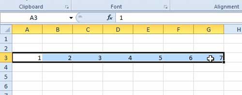
Step 2: Use your mouse to highlight the cells for which you wish to find a sum.

Step 3: Click the Home tab at the top of the window.

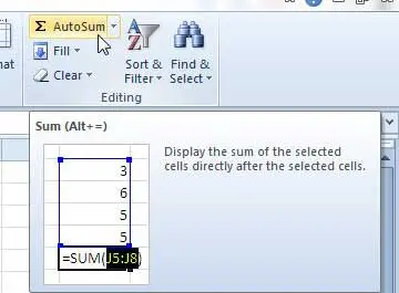
Step 4: Click the AutoSum button in the Editing section of the ribbon.

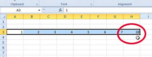
The sum of the selected cells will be displayed in the cell to the right, as in the image below.

Now that you know how to find a row sum in Excel 2010, you can use this formula to easily add values in other spreadsheets and cell ranges as well.
If you wish to manually enter the formula that adds your cells together, the formula is =SUM(XX:YY) where XX is the first cell, and YY is the last cell. For example, in my example above, the formula would be =SUM(A3:G3). Manual entry is a better option if you need to display the sum value in a cell that is not directly to the right of the row cells that you want to add.
Can I Use the Sum Formula By Manually Entering Cell References?
As we mentioned in the previous paragraph, you don’t need to rely on using your mouse to select cells for your autosum formula.
The Excel autosum will still sum numbers in your spreadsheet as long as the structure of the formula appears accurately. So whether the values in the formula got there by you selecting the cells yourself or entering them manually, then the only thing that matters is whether all of the parts of the formula are correct.
If Excel is telling you that an error occurred after you include all of your values in the formula then you may want to try using your mouse to select the cell and enter the Autosum formula. Since this will create the correct formula automatically you can see how it should look, which can help to determine where the error exists in the formula that you typed manually.
Will the Sum Function Only Include Visible Cells?
When you use your mouse to select a group of adjacent cells, you are also going to be selecting any hidden cells within that range of cells.
If you don’t want to include all the cells in a range when you create a SUM function, Excel requires you to use the same formula, just with a minor adjustment. The following formula will allow you to determine numeric values for more than one cell that aren’t in adjacent columns.
=SUM(XX,YY,ZZ)
Note that the equal sign and the autosum function are the same, but you need to format the referenced range a little differently.
Rather than using a colon to separate the first and the last values of the range you are going to enter the function manually with a comma between each cell that you want to sum.
Once you have added all of the cell references that you wish to auto sum then you can press Enter on your keyboard to execute the formula.
If you don’t want to type each cell individually then you can enter the =SUM( part of the formula, then you can click the first cell to include in the Excel sum, then hold down the Ctrl key on your keyboard and click on each additional cell to include in the formula. Each selected cell will have a dotted line around its cell after you select it.
Once you are finished clicking on each cell to include you can check the formula bar above the spreadsheet to determine that you have the correct range, then add the closing parenthesis to the end of the formula.
More Information on How to Find a Row Sum in Excel 2010
The steps in this article have shown you a way to determine the sum of values in a row of your spreadsheet. However, these same steps can also be used if you want to know how to find the sum of a column in Excel. You would simply need to select the column values instead.
While using a button in the ribbon is an efficient way to apply the Sum formula to a selection, you can manually type it into a cell as well.
If you click on the cell where you wish to display the sum of the values you can type this formula:
=SUM(XX:YY)
Where XX is the first cell in the range that you wish to add, and YY is the last cell in the range that you want to add.
If you want to get a sum for multiple ranges in a group of rows or columns then you only need to adjust your selection to include those ranges. For example, if I wanted to get a running total of the values in column c and column d of my spreadsheet then I would only need to enter the =SUM( part of my formula into the cell where I want to display the total, then click on the topmost cell to include in the range in column c and drag my mouse down until all of the desired cells are included in the selection. You would then type the closing parenthesis to complete the formula.
If you have a Netflix or Amazon Prime account and you want to watch it on your TV, then the Roku LT is the simplest and most affordable option available. Click here to learn more about the Roku LT.
Learn how to compare values in columns in Excel 2010.

Matthew Burleigh has been writing tech tutorials since 2008. His writing has appeared on dozens of different websites and been read over 50 million times.
After receiving his Bachelor’s and Master’s degrees in Computer Science he spent several years working in IT management for small businesses. However, he now works full time writing content online and creating websites.
His main writing topics include iPhones, Microsoft Office, Google Apps, Android, and Photoshop, but he has also written about many other tech topics as well.