You might discover that you need to know how to remove leading spaces in Excel when you have data that is difficult to work with and you can’t figure out why.
Sorting data alphabetically is a very useful ability that can make the information in your Excel worksheet easier to understand.
But occasionally you will sort data, only to wind up with a confusing arrangement of cells that do not seem to be sorted properly. Often this can occur because of spaces that exist before the actual data in the cell.
Manually deleting these spaces can be tedious, especially if you have a lot of cells that you need to fix. Our guide below will show you how to use the TRIM formula to remove leading spaces from cells in Microsoft Excel 2013.
If you need to remove letters or numbers from cells instead, then our guide on how to remove first character in Excel will show you how to accomplish that.
How to Trim Leading Spaces in Excel 2013
The steps in this article will show you how to remove spaces that exist before the data in your cell. We will accomplish this with the help of the TRIM formula.
Note that this will also delete any extra spaces between words in your data, as well as any spaces that appear after the data.
Step 1: Open your workbook in Excel 2013.
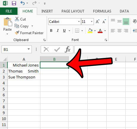
Step 2: Click inside the cell where you want to display the trimmed data.

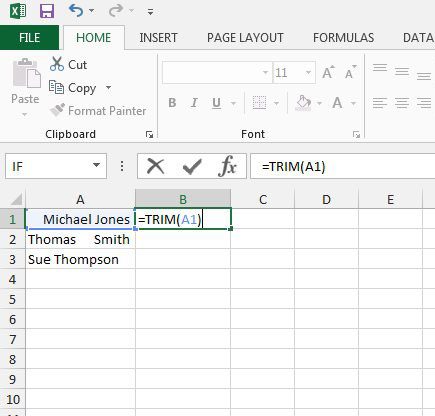
Step 3: Type the formula =TRIM(XX) where XX is the location of the data that you want to trim. In the example image below, this is cell A1.

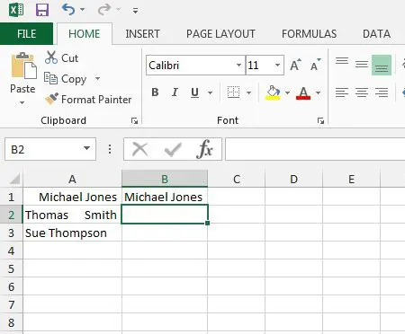
Step 4: Press the Enter key on your keyboard to execute the formula.

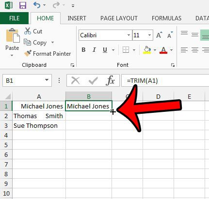
If you wish to apply this formula to the rest of the data in the same column, then click the fill handle at the bottom-right corner of the cell containing the formula that you just typed, then drag it down until you have selected an equal number of cells as those that you wish to trim.

Summary – How to remove leading spaces in Excel 2013
- Open your workbook in Excel 2013.
- Click inside the cell where you want to display the trimmed data. This must be a different cell than the one in which the data is currently located.
- Type the formula =TRIM(XX) where XX is the cell location that contains the data you want to trim.
- Press Enter on your keyboard to execute the trim formula.
If you are planning to then replace the original data with the trimmed data, you will need to paste the trimmed data into the original cells as values, instead of using the basic copy and paste procedure. Otherwise you may wind up with a column of cells that all say #REF!. Learn more about pasting as values in Excel and see some additional options that can make it easier to move data between different worksheets and workbooks.

Matthew Burleigh has been writing tech tutorials since 2008. His writing has appeared on dozens of different websites and been read over 50 million times.
After receiving his Bachelor’s and Master’s degrees in Computer Science he spent several years working in IT management for small businesses. However, he now works full time writing content online and creating websites.
His main writing topics include iPhones, Microsoft Office, Google Apps, Android, and Photoshop, but he has also written about many other tech topics as well.