How to Change Border Color in Excel 2010

Microsoft Excel 2010 is an almost infinitely customizable program. Aside from being able to choose, edit and modify every cell in your spreadsheet, you can also set options for how the cells are displayed.

This does not apply to only the data in the cells, however. You can also customize the way that the cells themselves look.

This includes providing you with the means to learn how to change border colors in Excel 2010. If, for example, you wanted to print or display your cells with a border color other than black, Excel 2010 allows you to do so.

The method for changing border colors in Excel 2010 is found on the Format Cells menu and gives you multiple options for choosing how to color your cell borders.

Microsoft Excel – Change Border Color

1. Open the spreadsheet.
2. Select the cells with borders.
3. Right-click a selected cell and choose Format Cells.
4. Choose the Border tab.
5. Click the Color drop down and select the desired color.
6. Click OK.

Our guide continues below with more information on changing border color in Microsoft Excel, including pictures of these steps.

How to Color Cell Borders in Excel 2010 (Guide with Pictures)

If you elect to combine cell border colors with cell fill colors, you will probably be able to come up with some pretty interesting effects.

Aside from simply improving the appearance of your spreadsheet, this can also be a helpful way to sort and organize your information.

Regardless of your intentions, you can easily learn how to change the border colors of cells in Excel 2010 using the steps outlined below.

Step 1: Open the spreadsheet containing the cells for which you want to change the border color.

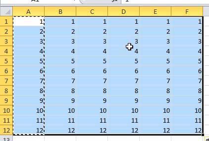
Step 2: Use your mouse to select the cells whose border colors you want to change.

You can also click the cell at the top-left corner of the spreadsheet between the row 1 and column A headings to select all of the cells in the worksheet.

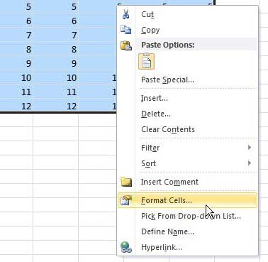
Step 3: Right-click the highlighted cells, then choose the Format Cells option.

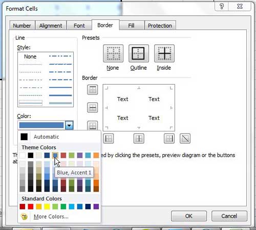
Step 4: Click the Border tab at the top of the window to display the cell border customization menu.

Step 5: Click the drop-down menu under Color, then choose the color that you want to use for your cell borders.

You can also select a line style from the window at the left side of the window.

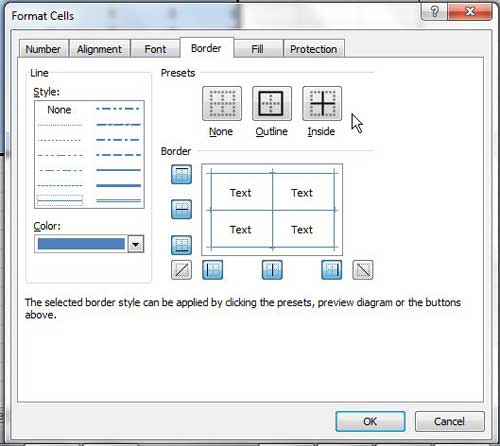
Step 6: Choose the border styles you want to use under Presets at the top of the window.

Now that you know how to change border color in Excel 2010, you can use this option anytime that you have borders around a cell that you need to switch to a different color.

If you want to highlight the borders of each individual cell, choose both the Outline and Inside options.

Once all of your border color settings have been established, click the OK button at the bottom of the window to apply the changes.

It is important to follow the steps in this order to set your border colors; otherwise, Excel 2010 will continue to apply a black border to the cells.

Is There Another Way to Open the Format Cells Dialog Box?

The Format Cells window that opens when you right-click a cell and then click Format Cells can be opened in other ways, too.

One of the simpler ways is to click the small Font Settings button at the bottom-right corner of the Font group.

Once that dialog box is open, you can simply click the Borders tab, where you will be able to change the border type, line color and generally just add borders and adjust their settings.

More Information on How to Change Border Color in Excel

While the steps in this guide will show you how to change the cell outline color, it’s important that you have first enabled the borders for the cells where you will be changing the cell border color. You can do this by selecting the cells in the spreadsheet, then clicking the down arrow next to the Border button, and choosing the All Borders option.

You can remove cell borders and the cell border color by selecting the cells with the color, then clicking the arrow next to the Borders button and choosing the No Border option.

One other way that you can get to the menu where you change cell border colors is to click the Borders arrow, then choose the More Borders option at the bottom of the drop-down list. This method also opens the “Format Cells” window and can be a little easier to remember if you don’t often use the right-click option in applications.

There can be some confusion concerning Excel borders and gridlines. The gridlines in a spreadsheet are shown by default and identify the separation between rows and columns. Borders are a formatting option that you can add to your selected cells.

If you select cells with borders, then click the Clear button in the Editing group and choose Clear Formats, then it will remove the cell borders. However, the gridlines will remain. To remove gridlines, you need to click the Page Layout tab, then uncheck the options under Gridlines.

Another interesting option that you may find useful involves creating a cell style. You can do this by selecting the Home tab, then clicking Cell Styles in the Styles group of the ribbon. You will then be able to click cell styles that are pre-defined, or you can create a new cell style. When creating a new cell style, you have a variety of display options that you can add to the style. You may also wish to define a name in the Style Name box to make it easier to identify in the future.

Once you have an existing cell style, you can select multiple cells or a range of cells in your spreadsheet, then simply apply one of the existing styles to that selection.