How to Create a Named Range in Google Sheets

You can create a named range in a Google spreadsheet by selecting the cells for the range, clicking the Data tab and choosing Named ranges, then typing a name and clicking Done.

I have been working with spreadsheets in Microsoft Excel and Google Sheets for a long time, and have grown accustomed to doing things a certain way.

This is particularly true when making formulas, as it’s very easy to make a mistake with the structure of the formula, so I tend to always do things the same way.

One particular option I learned to be helpful, however, is providing a name to a range of cells that you will be referencing a lot.

This can speed up a lot of formula creation, while also ensuring that you include everything you need.

Our tutorial below will show you how to create a named range in Google Sheets.

How to Give a Name to a Range in a Google Spreadsheet

1. Open your Google Sheets spreadsheet.
2. Highlight the range of cells.
3. Click the Data tab and choose Named ranges.
4. Type a name for the range and click Done.

Our guide continues below with additional information on how to create a named range in Google Sheets, including pictures of these steps.

Formulas are a fantastic feature in spreadsheet applications that allow you to quickly perform mathematical operations on cells.

The nature of these formulas even makes it so that you can change a value in one of those cells, and it will automatically update the result of the formula.

Typically you need to define a range of cells when you use a formula, but a feature called Named ranges can make that step a little simpler if you want to save yourself some time with ranges that you use a lot.

Our guide below will show you how to create and use a Named range in the Google Sheets application.

When you need to compare values in an Excel spreadsheet but aren’t sure about the syntax for the formulas, view our Excel subtraction formula guide for more information.

How to Set a Google Sheets Named Range (Guide with Pictures)

The steps in this article are going to show you how to create a named range in a Google Sheets spreadsheet from a group of existing data in that sheet.

You will then be able to refer to that named range by the name that you create when you use it in formulas.

Find out how to merge cells in Google Sheets if you have done so in Excel, but are having trouble finding the option in Google’s spreadsheet app.

Step 1: Go to your Google Drive at https://drive.google.com/drive/my-drive and open the spreadsheet containing the data that you want to set as a named range.

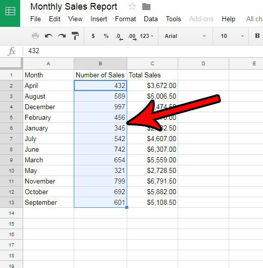
Step 2: Select the cells containing the data for the named range.

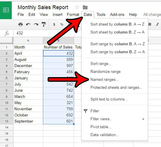
Step 3: Click the Data option at the top of the window, then click the Named ranges option.

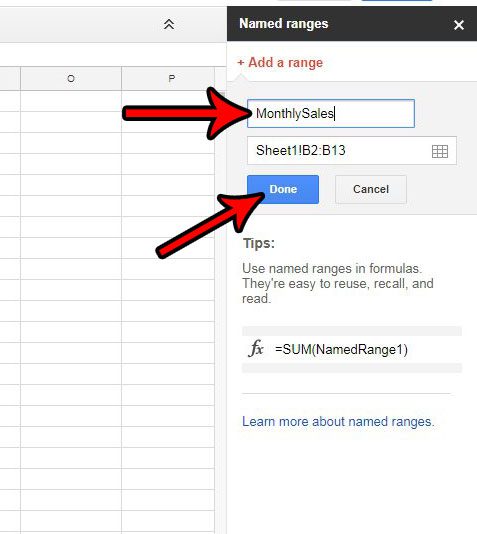
Step 4: Enter a name for the named range into the top field of the column at the right side of the window, then click the Done button.

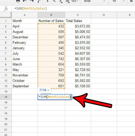
Step 5: You can then use this named range in place of the cell references that you have previously been using in formulas.

For example, in the image below I can get a sum of the named range by typing =SUM(MonthlySales) into a cell, rather than the =SUM(B2:B13) formula I would have had to use before.

This can be a real time-saver if you have to reuse the same range of cells in multiple formulas, or if the range takes a while to select.

Now that you know how to create a named range in Google Sheets, you can use this technique to make it easier for you to perform a number of different actions within your spreadsheets.

Does your school or job require you to submit Excel files, but you don’t have Excel? Learn how to export Excel files from Google Sheets using a quick process.